Natural Language Processing (NLP) MSc IT - Sem IV - As per Mumbai University Syllabus


Unit - 1
Chapter: 1

Introduction to NLP, Brief history, NLP applications: Speech To Text (STT) / Speech Recognition, Text to Speech (TTS), Story Understanding, NL Generation /Conversation systems – Dialog Systems / Chatbots, QA system, Machine Translation / Language Translation, challenges/Open Problems, NLP abstraction levels, Natural Language (NL) Characteristics, NL computing approaches / techniques and steps.
NL tasks: Segmentation, Chunking, tagging, NER (Named Entity Recognition), Parsing, Word Sense Disambiguation, NL Generation, 


Web 2.0 Applications : Sentiment Analysis, Text Entailment, Cross Lingual Information Retrieval (CLIR)

Chapter: 2


Text Preprocessing
Introduction, Challenges of Text Pre-processing, Word Level -Tokenization, Sentence Segmentation


Chapter 3: 


Lexical Analysis
Basic word classes (parts of speech), Word Formation Processes, Finite State Morphonology, Two level morphology, “Difficult” Morphology and Lexical Analysis


Introduction to NLP

Natural Language Processing (NLP) is basically how you can teach machines to understand human languages and extract meaning from text.
Language as a structured (grammatical) medium of communication is what separates us human beings from animals. 
We are surrounded by text data all the time sourced from books, emails, blogs, social media posts, news and more. 

Dataset Types: Structured and Unstructured

Structured datasets

Data having fix number of dimensions – that is fixed number of keys and its values, or fixed number of rows and columns is called a structured dataset. 
This type of dataset contains information in a well-organized form.
Generally,  a structure dataset is present in a tabular format like  relational databases- as shown, where dimension of dataset is fixed, or it is in a key-value pair-json file showing students marks in key-value pairs.

Unstructured datasets

Unstructured dataset lacks a particular structure i.e. no structure  
It doesn’t have fixed dimensions i.e. it can take any form
For example- audios, videos, images and text 
Images 
Video recording of road highway
These images and videos are processed by computers and converted to long text of bits and bytes, which human can’t identify the right information or context.
 so, it cannot be well designed in a tabular format
Text dataset
Examples of text data:
Social media data: tweets, posts, comments
Conversation data: messages, emails, chats
Articles:  news, blogs, transcripts 
So, a text data is essentially any written form of Natural language such as English, Russian or Japanese.
It consists of characters or words arranged together in a meaningful and a formal manner, which means that text data is driven by the grammar rules and defined structures 

Introduction to Natural Language Processing (NLP)

NLP is the branch of Data Science, which deals with deriving useful information from the text data / Natural Language Text
Also known as Computational Linguistics (CL), Human Language Technology (HLT), Natural Language Engineering (NLE)
It contains several different techniques and processes which are used to analyze, understand and utilize the text data for solving business needs.
Often, we come across a term Applied NLP.
Applied NLP: NLP + Human Interaction.
Which means, the use of NLP for designing and developing applications or systems in which there exists an interaction between machines and  natural languages.   

History of natural language processing


Applications of Natural Language Processing

Speech To Text (STT) / Speech Recognition
Text to Speech (TTS)
Story Understanding
NL Generation /Conversation systems – Dialog Systems / Chatbots
QA system
Machine Translation / Language Translation
Text Summarizers
Text Classification
Sentiment Analysis
Grammar / spell check / Autocorrect
1: Speech To Text (STT) / Speech Recognition
Speech to text conversion is the process of converting spoken words into written texts. 
This process is also often called speech recognition. 
All speech-to-text systems rely on at least two models: an acoustic model and a language model. In addition large vocabulary systems use a pronunciation model. 
To get the best transcription quality, all of these models can be specialized for a given language, dialect(idioms), application domain, type of speech, and communication channel. 
Application: dictate in word or power point

2: Text to Speech (TTS)
Text-to-speech (TTS) is a type of  assistive technology that reads digital text aloud. It’s sometimes called “read aloud” technology.
The voice in TTS is computer-generated, and reading speed can usually be speed up or slowed down.
Some TTS tools also have a technology called optical character recognition (OCR). 
OCR allows TTS tools to read text aloud from images. 
For example, person could take a photo of a street sign and have the words on the sign turned into audio.
Application: ebook reader

3: Story Understanding
A large body of work in story understanding has focused on learning scripts.
Scripts represent structured knowledge about stereotypical event, sequences together with their participants.
‘A narrative or story is anything which is told in the form of a causally (logically) linked set of events involving some shared characters’.
Instead of predicting an event, the system is tasked with choosing an entire sentence to complete the given story.
Application: Story Wizard

4: NL Generation
Natural Language Generation (NLG) is the process of generating descriptions or narratives in natural language from structured data.
NLG often works closely with Natural Language Understanding (NLU).
NLG, along with NLU, is at the core of chatbots and voice assistants.
For computer science domain, NLG has been used to write specifications from UML diagrams, or describe source code changes.
Application: Tableau

5: QA systems
It is used to answer questions in the form of natural language and has a wide range of applications. 
Typical applications include: intelligent voice interaction, online customer service, knowledge acquisition, personalized emotional chatting, and more. 
There are two types of QA systems, open and closed. 
A system that tries to answer any question you could possibly ask is called an open system or open domain system – think of Google or Alexa.
And then there are closed (or closed domain) systems that are built for a certain subject or function or domain of knowledge or company. E.g. Paypal, Finn AI, Digital genius etc.

6: Machine Translation (MT) 
Machine Translation (MT) is the task of automatically converting one natural language into another, preserving the meaning of the input text, and producing fluent text in the output language. 
There are many challenging aspects of MT: 
the large variety of languages, alphabets and grammars; 
the task to translate a sequence (a sentence for example) to a sequence is harder for a computer than working with numbers only; 
there is no one correct answer 
Application: google translator 

7: Text Summarization 
It is a process of generating a concise and meaningful summary of text from multiple text resources such as books, news articles, blog posts, research papers, emails, and tweets.
Text summarization can broadly be divided into two categories — Extractive Summarization  and Abstractive Summarization.
Extractive Summarization: These methods rely on extracting several parts, such as phrases and sentences, from a piece of text and stack them together to create a summary. E.g. Text-Processing, Skyttle 2.0, Textuality.
Abstractive Summarization: These methods use advanced NLP techniques to generate an entirely new summary. Some parts of this summary may not even appear in the original text. E.g. Digital Tesseract

8: Text classification 
Text classification also known as text tagging or text categorization is the process of categorizing text into organized groups.
By using NLP, text classifiers can automatically analyse text and then assign a set of pre-defined tags or categories based on its content.
Unstructured text is everywhere, such as emails, chat conversations, websites, and social media but it’s hard to extract value from this data unless it’s organized in a certain way. 
Text classifiers with NLP have proven to be a great alternative to structure textual data in a fast, cost-effective, and scalable way.
Application: Email services / medical report / news

9: Sentiment analysis / opinion mining
Sentiment analysis (or opinion mining) is a NLP technique used to determine whether data is positive, negative or neutral. 
Sentiment analysis is often performed on textual data to help businesses monitor brand and product sentiment in customer feedback, and understand customer needs.
Sentiment analysis models focus on polarity (positive, negative, neutral) and also on feelings and emotions (angry, happy, sad, etc), urgency (urgent, not urgent) and even intentions (interested v. not interested).
Application: pros and cons of a product – useful in e-commerce

10: Grammar / spell check / Autocorrect
A word needs to be checked for spelling correctness and corrected if necessary, many a time in the context of the surrounding words. 
Spell Check is a process of detecting and sometimes providing suggestions for incorrectly spelled words in a text.
A basic spell checker carries out the following processes: 
It scans the text and extracts the words contained in it. 
It then compares each word with a known list of correctly spelled words (i.e. a dictionary).
Application: word /power point / google search
Autocorrect
 
Business Use cases of NLP 
- A “Use case” is the theoretical side of an “Application”

Business Use case 1
Example of smartphone brand to find most relevant and consumer and audience preferences about the smartphones, which will help them improve the sales of their new smartphone model.
Analyze: social media data
Identify: most talked issues, sentiments
Model: causes of negative sentiments

Business use case 2
Take the example of telecom company who wants to categorize the customer queries to respective departments. 
This way the company can reduce the time taken to resolve a customer query
The company found out that most of the time goes in identification of department, which is most relevant to the given customer query.
The company can analyze top keywords and phrases of the query  
They can map those keywords and phrases with the description of respective department.
Finally, they can come up with the model or business rules for automatic categorization and assignment of queries to the respective department.

Business Use case 3
Identify patients at Risk of Cancer
The hospital can analyse the history of patient, which includes diseases, and drugs prescribed to them in the past. The data used in this process used in this process will be doctor notes, patient prescriptions and other past medical reports.
The hospital can identify key entities from the patient history, such as the need of the drugs prescribed to them in the past, or the symptoms the patient has shown in the past. 
This information can be modelled together using business rules, to classify the risk level of the patient.

Challenges/Open Problems
Contextual words and phrases and homonyms
Synonyms
Irony and sarcasm
Ambiguity
Errors in text and speech
Colloquialisms(idioms) and slang (a form of informal language)
Domain-specific language

1) Contextual words and phrases and homonyms
The same words and phrases can have different meanings according the context of a sentence and many words – especially in English – have the exact same pronunciation but totally different meanings.
For example:
I ran to the store because we ran out of milk.
More example of homonyms: 
Address - to speak to / location
Bright - very smart or intelligent / filled with light
Kind - type / caring

2) Synonyms
Synonyms can lead to issues similar to contextual understanding because we use many different words to express the same idea. Furthermore, some of these words may convey exactly the same meaning, while some may be levels of complexity (small, little, tiny, minute) and different people use synonyms to denote slightly different meanings within their personal vocabulary.
So, for building NLP systems, it’s important to include all of a word’s possible meanings and all possible synonyms. 

3) Irony and sarcasm
Irony is usually delivered as a joke (Describing someone who says foolish things a “genius”) while sarcasm is delivered with a hint of anger (I’m not insulting you. I’m just describing you.). 
Irony and sarcasm present problems for machine learning models because they generally use words and phrases that, strictly by definition, may be positive or negative, but actually imply the opposite.
Models can be trained with certain cues that frequently accompany ironic or sarcastic phrases, like “yeah right,” “whatever,” etc., 

4) Ambiguity
Ambiguity in NLP refers to sentences and phrases that potentially have two or more possible interpretations.
Lexical ambiguity: a word that could be used as a verb, noun, or adjective.
    e.g. back; noun - he stood at the back of the stage; verb - The car backed up and hit the tree;   adjective - the back entrance
Semantic ambiguity: the interpretation of a sentence in context. For example: I saw the boy on the beach with my binoculars. This could mean that I saw a boy through my binoculars, or the boy had my binoculars with him
Syntactic ambiguity: In the sentence above, this is what creates the confusion of meaning. The phrase with my binoculars could modify the verb, “saw,” or the noun, “boy.”

5) Errors in text and speech
Misspelled or misused words can create problems for text analysis. Autocorrect and grammar correction applications can handle common mistakes, but don’t always understand the writer’s intention.

6) Colloquialisms and slang
Informal phrases, expressions, idioms, and culture-specific lingo(language / speech) present a number of problems for NLP – especially for models intended for broad use. 
Because as formal language, colloquialisms may have no “dictionary definition” at all, and these expressions may even have different meanings in different geographic areas. Furthermore, cultural slang is constantly morphing and expanding, so new words pop up every day.

7) Domain-specific language
Different businesses and industries often use very different language. An NLP processing model needed for healthcare, for example, would be very different than one used to process legal documents. 

NLP abstraction levels
Tokenization and sentence segmentation
Lexical analysis
Syntactic Analysis
Semantic Analysis
Pragmatic Analysis
Tokenization and sentence segmentation: Natural language text is generally not made up of the short, neat, well-formed, and well-delimited sentences.
Tokenization and sentence segmentation So, we need to separate all individual tokens having the “minimal unit of meaning”, is referred to as the morpheme. E.g. happiness The stem happy is considered as a free morpheme since it is a “word” in its own. Bound morphemes (prefixes and suffixes) require a free morpheme to which it can be attached to and can therefore not appear as a “word” on their own.

Lexical analysis: The lexical analysis in NLP deals with the study at the level of words with respect to their lexical (word) meaning and part-of-speech. This level of linguistic processing utilizes a language’s lexicon (dictionary), which is a collection of individual lexemes. A lexeme is a basic unit of lexical meaning; which is an abstract unit of morphological analysis that represents the set of forms or “senses” taken by a single morpheme.
“duck”, for example, can take the form of a noun (swimming bird) or a verb (bow down) but its part-of-speech and lexical meaning can only be derived in context with other words used in the phrase/sentence. This, in fact, is an early step towards a more sophisticated Information Retrieval system where precision is improved through part-of-speech tagging.


Syntactic Analysis: Syntactic Analysis also referred to as “parsing”, allows the extraction of phrases which convey more meaning than just the individual words by themselves. In Information Retrieval, parsing can be forced to improve indexing since phrases can be used as representations of documents which provide better information than just single-word indices. In the same way, phrases that are syntactically derived from the query offers better search keys to match with documents that are similarly parsed.
      Nevertheless, syntax can still be ambiguous at times as in the case of the news headline: “Boy paralyzed after tumour fights back to gain black belt” — which actually refers to how a boy was paralyzed because of a tumour but endured the fight against the disease and ultimately gained a high level of competence in martial arts.


Semantic Analysis: understand meaning of syntactically correct tokens or statements.
      The semantic level of linguistic processing deals with the determination of what a sentence really means by relating syntactic features and disambiguating words with multiple definitions to the given context. This level entails the appropriate interpretation of the meaning of sentences, rather than the analysis at the level of individual words or phrases.


Pragmatic Analysis: The pragmatic(Realistic / Logical) level of linguistic processing deals with the use of real-world knowledge and understanding of how this impacts the meaning of what is being communicated. By analyzing the contextual dimension of the documents and queries, a more detailed representation is derived.
In Information Retrieval, this level of Natural Language Processing primarily engages query processing and understanding by integrating the user’s history and goals as well as the context upon which the query is being made. Contexts may include time and location.
This level of analysis enables major breakthroughs in Information Retrieval as it facilitates the conversation between the information retrieval system and the users, allowing the induction of the purpose upon which the information being sought is planned to be used, thereby ensuring that the information retrieval system is fit for purpose.

Natural Language (NL) Characteristics 
Language is Arbitrary
Language is Social
Language is Symbolic
Language is Systematic
Language is Vocal
Language is Non-instinctive(instinct – natural / unlearn) 
Language is Productive and Creative
Language is Arbitrary: Language is arbitrary in the sense that there is no inherent relation between the words of a language and their meanings or the ideas conveyed by them.
Language is Social: Language is a set of conventional communicative signals used by humans for communication in a community.
Language is Symbolic: Language consists of various sound symbols and their graphological counterparts that are employed to denote some objects, occurrences or meaning.  

Language is Systematic: Although language is symbolic, yet its symbols are arranged in a particular system.  All languages have their system of arrangements. Furthermore, all languages have phonological and syntactic systems and within a system, there are also several sub-systems.
Language is Vocal: 
      Language is primarily made up of vocal sounds only produced by a physiological articulatory mechanism (accent) in the human body.
      Writing is only the graphic representation of the sounds of the language.

Language is Non-instinctive(instinct – natural / unlearn): 
No language was created in a day out of a mutually agreed upon formula by a group of humans. 
Language is the outcome of evolution and convention. 
Each generation transmits this convention on to the next.

Language is Productive and Creative: 
Language has creativity and productivity.
The structural elements of human language can be combined to produce new utterances(words), which neither the speaker nor his hearers may ever have made or heard before any, listener, yet which both sides understand without difficulty.

NL computing approaches / techniques and steps

1. Text Pre-processing(Tokenization):
Not all languages deliver text in the form of words neatly delimited by spaces.
It is of crucial importance to ensure that, given a text, we can break it into sentence-sized pieces.

2. Lexical Analysis:
Decomposing words into their parts and maintaining rules for how combinations are formed.
morphological processing can go some way toward handling unrecognized words.
Morphological processes alter stems to derive new words. They may change the word’s meaning (derivational) or grammatical function (inflectional).

3. Syntactic Parsing:
The basic unit of meaning analysis is the sentence: a sentence expresses a proposition, an idea, or a thought, and says something about some real or imaginary world.
In NLP approaches based on generative linguistics, this is generally taken to involve the determining of the syntactic or grammatical structure of each sentence.

4. Semantic Analysis:
It is these subsequent steps that derive a meaning for the sentence in question.

5. Natural Language Generation:
In many situations, a response then needs to be generated, either in natural language alone or in combination with other modalities.

NLP Terminology

Phonology − It is study of organizing sound systematically.
Morpheme − A meaningful linguistic unit that cannot be divided into smaller meaningful parts..
Syntax − It refers to arranging words to make a sentence. It also involves determining the structural role of words in the sentence and in phrases.
Semantics − It is concerned with the meaning of words and how to combine words into meaningful phrases and sentences.
Pragmatics − It deals with using and understanding sentences in different situations and how the interpretation of the sentence is affected with reference to the context.
Discourse − It deals with how the immediately preceding sentence can affect the interpretation of the next sentence.
Corpus -  A corpus is a large and structured set of machine-readable texts that have been produced in a natural communicative setting. Corpora is the plural of corpus . They can be derived in different ways like text that was originally electronic, transcripts of spoken language and optical character recognition, etc.

NL tasks: 
Segmentation 
Text segmentation is the process of dividing written text into meaningful units, such as words, sentences, or topics. The term applies both to mental processes used by humans when reading text, and to artificial processes implemented in computers, which are the subject of natural language processing.
Word segmentation - Word segmentation is the problem of dividing a string of written language into its component words.
Intent segmentation - Intent segmentation is the problem of dividing written words into key phrases (2 or more group of words).
Sentence segmentation - Sentence segmentation is the problem of dividing a string of written language into its component sentences.
Topic segmentation - Topic analysis consists of two main tasks: topic identification and text segmentation. While the first is a simple classification of a specific text, the latter case implies that a document may contain multiple topics, and the task of computerized text segmentation may be to discover these topics automatically and segment the text accordingly. The topic boundaries may be apparent from section titles and paragraphs. In other cases, one needs to use techniques similar to those used in document classification.
Segmenting the text into topics or discourse turns might be useful in some natural processing tasks: it can improve information retrieval or speech recognition significantly (by indexing/recognizing documents more precisely or by giving the specific part of a document corresponding to the query as a result). It is also needed in topic detection and tracking systems and text summarizing problems.

Tagging
POS Tagging (Parts of Speech Tagging) is a process to mark up the words in text format for a particular part of a speech based on its definition and context. It is responsible for text reading in a language and assigning some specific token (Parts of Speech) to each word. It is also called grammatical tagging.
For example: 
Input: Everything to permit us.
Output: [('Everything', NN),('to', TO), ('permit', VB), ('us', PRP)]
Steps Involved in the POS tagging example:
Tokenize text (word_tokenize)
apply pos_tag to above step that is nltk.pos_tag(tokenize_text)


Chunking
Chunking in NLP is a process to take small pieces of information and group them into large units. The primary use of Chunking is making groups of "noun phrases." It is used to add structure to the sentence by following POS tagging combined with regular expressions. The resulted group of words are called "chunks." It is also called shallow parsing.
In shallow parsing, there is maximum one level between roots and leaves while deep parsing comprises of more than one level. Shallow parsing is also called light parsing or chunking.

Rules for Chunking:
There are no pre-defined rules, but you can combine them according to need and requirement.
For example, you need to tag Noun, verb (past tense), adjective, and coordinating conjunction(e.g. and, but..) from the sentence. You can use the rule as below
chunk:{<NN.?>*<VBD.?>*<JJ.?>*<CC>?}


Following table shows what the various symbol means:

#Example:
from nltk import pos_tag
from nltk import RegexpParser
text ="learn NLP from NPTEL and make study easy".split()
print("After Split:",text)
import nltk
nltk.download('averaged_perceptron_tagger')
tokens_tag = pos_tag(text)
print("After Token:",tokens_tag)
patterns= """mychunk:{<NN.?>*<VBD.?>*<JJ.?>*<CC>?}"""
chunker = RegexpParser(patterns)
print("After Regex:",chunker)
output = chunker.parse(tokens_tag)
print("After Chunking",output)
Output
After Split: ['learn', 'NLP', 'from', 'NPTEL', 'and', 'make', 'study', 'easy’]

After Token: [('learn', 'JJ'), ('NLP', 'NNP'), ('from', 'IN'), ('NPTEL', 'NNP'), ('and', 'CC'), ('make', 'VB'), ('study', 'NN'), ('easy', 'JJ’)]

After Regex: chunk.RegexpParser with 1 stages: RegexpChunkParser with 1 rules: <ChunkRule: '<NN.?>*<VBD.?>*<JJ.?>*<CC>?’>

After Chunking (S 
  mychunk learn/JJ) 
  mychunk NLP/NNP) 
  from/IN 
  mychunk NPTEL/NNP and/CC) 
  make/VB 
  mychunk study/NN easy/JJ))

Chunking is used for entity detection. An entity is that part of the sentence by which machine gets the value for any intention.
Example: 
Temperature of India. 
Here Temperature is the intention and India is an entity. 
In other words, chunking is used as selecting the subsets of tokens. 

NER (Named Entity Recognition)
Named entity recognition (NER) is one of the most common uses of Information Extraction (IE) technology.
NER systems identify different types of proper names, such as person and company names, and sometimes special types of entities, such as dates and times, that can be easily.  
NER is especially important in biomedical applications, where terminology is a formidable (difficult) problem. But IE is much more than just NER. 

A much more difficult and potentially much more significant capability is the recognition of events and their participants. 
For example, in each of the sentences 
“Microsoft acquired Powerset.” 
“Powerset was acquired by Microsoft.” 
we would like to recognize not only that Microsoft and Powerset are company names, but also that an acquisition event took place, that the acquiring company was Microsoft, and the acquired company was Powerset. 


How Does Named Entity Recognition Work?
When we read a text, we naturally recognize named entities like people, organization name, locations, and so on. For example, in the sentence “Mark Zuckerberg is one of the founders of Facebook, a company from the United States” we can identify three types of entities:
“Person”: Mark Zuckerberg
“Company”: Facebook
“Location”: United States


For computers, however, we need to help them recognize entities first so that they can categorize them.
This is done through machine learning and Natural Language Processing (NLP).
NLP studies the structure and rules of language and creates intelligent systems capable of deriving meaning from text and speech, while machine learning helps machines learn and improve over time.
To learn what an entity is, an NER model needs to be able to detect a word, or string of words that form an entity (e.g. New York City) and know which entity category it belongs to.


So first, we need to create entity categories, like Name, Location, Event, Organization, etc., and feed NER model relevant training data. Then, by tagging some word and phrase samples with their corresponding entities, you’ll eventually teach your NER model how to detect entities itself.  
You may create entity extractor to extract people from a given corpus, or company name from a given corpus or any other entity.

Extracting the main entities in a text helps sort unstructured data and detect important information, which is crucial if you have to deal with large datasets.
Some interesting use cases of named entity recognition
Categorize Tickets in Customer Support: You can also use entity extraction to pull relevant pieces of data, like product names or serial numbers, making it easier to route tickets to the most suitable agent or team for handling that issue. 
Gain Insights from Customer Feedback: you could use NER to detect locations that are mentioned most often in negative customer feedback, which might lead you to focus on a particular office branch.

Content Recommendation: if you watch a lot of comedies on Netflix, you’ll get more recommendations that have been classified as the entity Comedy.
Process Resumes: By using an entity extractor, recruitment teams can instantly extract the most relevant information about candidates, from personal information (like name, address, phone number, date of birth and email), to data related to their training and experience (such as certifications, degree, company names, skills, etc).


How to use NER?
By adding a sufficient number of examples in the doc_list, one can produce a customized NER using spaCy.
spaCy supports the following entity types: PERSON, NORP (nationalities, religious and political groups), FAC (buildings, airports etc.), ORG (organizations), GPE (countries, cities etc.), LOC (mountain ranges, water bodies etc.), PRODUCT (products), EVENT (event names), WORK_OF_ART (books, song titles), LAW (legal document titles), LANGUAGE (named languages), DATE, TIME, PERCENT, MONEY, QUANTITY, ORDINAL and CARDINAL.
References
https://spacy.io/

Parsing
There is a significant difference between NLP and traditional machine learning tasks, with the former dealing with unstructured text data while the latter deals with structured tabular data. Hence, it is necessary to understand how to deal with text before applying machine learning techniques to it. This is where text parsing comes into the picture.
Text parsing is a common programming task that separates the given series of text into smaller components based on some rules. Its application ranges from document parsing to deep learning NLP.
Text parsing can be done with the two popular options are regular expressions and word tokenization.

An assumption in most work in natural language processing is that the basic unit of meaning analysis is the sentence: a sentence expresses a proposition(plan / suggestion) , an idea, or a thought, and says something about some real or imaginary world. 
Extracting the meaning from a sentence is thus a key issue. Sentences are not, however, just linear sequences of words, and so it is widely recognized that to carry out this task requires an analysis of each sentence, which determines its structure in one way or another. 
In NLP approaches based on generative linguistics, this is generally taken to involve the determining of the syntactic or grammatical structure of each sentence. 

Word Sense Disambiguation
We understand that words have different meanings based on the context of its usage in the sentence. If we talk about human languages, then they are ambiguous too because many words can be interpreted in multiple ways depending upon the context of their occurrence.
Word sense disambiguation, in NLP, may be defined as the ability to determine which meaning of word is activated by the given word in a particular context.
Lexical(word / vocabulary) ambiguity, syntactic or semantic, is one of the very first problem that any NLP system faces. 

Part-of-speech (POS) taggers with high level of accuracy can solve Word’s syntactic ambiguity. 
On the other hand, the problem of resolving semantic ambiguity is called WSD (word sense disambiguation). 
Resolving semantic ambiguity is harder than resolving syntactic ambiguity.
For example, consider the two examples of the distinct sense that exist for the word “bass” −
I can hear bass sound.
He likes to eat grilled bass.

The occurrence of the word bass clearly denotes the distinct meaning. 
In first sentence, it means frequency(low-pitched) and in second, it means fish. Hence, if it would be disambiguated by Word sense disambiguate(WSD) then the correct meaning to the above sentences can be assigned as follows −
I can hear bass/low-pitched frequency sound.
He likes to eat grilled bass/fish.

NL Generation
Natural language generation is one of the frontiers of artificial intelligence. It is the idea that computers and technologies can take non-language sources, for example, Excel spreadsheets, videos, metadata and other sources, and create natural language outputs that seem human, given that humans are the only biological creatures that use complex natural language.
NLG solutions are made of three main components: 
the data behind the narrative,
the conditional logic and  software that makes sense of that data, and 
the resulting content that is generated.

From video game and fantasy football match recaps, to custom BI dashboard analysis and client communications, natural language generation is valuable wherever there is a need to generate content from data.
Natural language generation empowers organizations to create data-driven narratives that are personalized, insightful, and sounds as if a human wrote each one individually—all at a massive scale.
NLG is different than NLP. NLP is focused on deriving analytic insights from textual data, NLG is used to synthesize textual content by combining analytic output with contextualized narratives.
In other words, NLP reads while NLG writes. NLP systems look at language and figure out what ideas are being communicated. NLG systems start with a set of ideas locked in data and turn them into language that, in turn, communicates them.

For example, using the historical data for July 1, 2005, the software produces:
Grass pollen levels for Friday have increased from the moderate to high levels of yesterday with values of around 6 to 7 across most parts of the country. However, in Northern areas, pollen levels will be moderate with values of 4.

How does NLG work?
An automated text generation process involves 6 stages. For the sake of simplicity, let’s consider each stage from an example of robot journalist news on a football match:
Content Determination: The limits of the content should be determined. The data often contains more information than necessary. In football news example, content regarding goals, cards, and penalties will be important for readers. 


Data interpretation: The analyzed data is interpreted. With machine learning techniques, patterns can be recognized in the processed data.  This is where data is put into context. For instance, information such as the winner of the match, goal scorers & assisters, minutes when goals are scored are identified in this stage.
Document planning: In this stage, the structures in the data are organized with the aim of creating a narrative structure and document plan. Football news generally starts with a paragraph that indicates the score of the game with a comment that describes the level of intensity and competitiveness in the game, then the writer reminds the pre-game standings of teams, describes other highlights of the game in the next paragraphs, and ends with player and coach interviews. 

Sentence Aggregation: It is also called micro planning, and this stage is where different sentences are aggregated in context because of their relevance. 
For example, below first two sentences provide different meanings. However, if the second event occurs right before half time, then these two sentences can be aggregated like the third sentence:
“[X team] maintained their lead into halftime. “
“VAR(virtual assistant referee) overruled a decision to award [Y team]’s [Football player Z] a penalty after replay showed [Football player T]’s apparent kick didn’t connect.”
“[X team] maintained their lead into halftime after VAR overruled a decision to award [Y team]’s [Football player Z] a penalty after replay showed [Football player T]’s apparent kick didn’t connect.”

Grammaticalization: Grammaticalization stage makes sure that the whole report follows the correct grammatical form, spelling, and punctuation. This includes validation of actual text according to the rules of syntax, morphology, and orthography.  For instance, football games are written in the past tense.
Language Implementation: This stage involves inputting data into templates and ensuring that the document is output in the right format and according to the preferences of the user. 

Web 2.0 Applications : Sentiment Analysis
Sentiment Analysis is the computational treatment of opinions, sentiments and subjectivity of text and use them for the benefit of the business operations.
It is the process of examining a piece of text for opinions and feelings. There are innumerable real-life use cases for sentiment analysis that include understanding how consumers feel about a product or service, looking for signs of depression, or to see how people respond to certain advertise and political campaigns.
There are three main classification levels in SA: 
document-level, 
sentence-level and 
aspect-level SA. 

Document-level SA aims to classify an opinion; whether the document as expressing a positive or negative opinion or sentiment. It considers the whole document a basic information unit.
Sentence-level SA aims to classify sentiment expressed in each sentence. The first step is to identify whether the sentence is subjective or objective. If the sentence is subjective, Sentence-level SA will determine whether the sentence expresses positive or negative opinions. 
Classifying text at the document level or at the sentence level does not provide the necessary detail needed in many applications. To obtain these details; we need to go to the aspect level. Aspect-level SA aims to classify the sentiment with respect to the specific aspects of entities. The first step is to identify the entities and their aspects.


It involves breaking down text data into smaller fragments, allowing you to obtain more granular and accurate insights from your data. 
For example: “The food was great but the service was poor.” 
In cases like this, there is more than one sentiment and more than one topic in a single sentence, so to label the whole review as either positive or negative would be incorrect. Use aspect-based sentiment analysis here, which extracts and separates each aspect and sentiment polarity in the sentence.
In this instance, the aspects are Food and Service, resulting in the following sentiment attribution:
The food was great = Food → Positive
The service was poor = Service → Negative

With the proper representation of the text after text pre-processing, many of the techniques, such as clustering and classification, can be adapted to text mining. 
For example, the k-means can be modified to cluster text documents into groups, where each group represents a collection of documents with a similar topic. 
The distance of a document to a centroid represents how closely the document talks about that topic. 
Classification tasks such as sentiment analysis and spam filtering are prominent use cases for the Naive Bayes classifier. Text mining may utilize methods and techniques from natural language processing.

Sentiment Analysis Steps

Text Entailment 
Textual entailment (TE- semantic interpretation) in natural language processing is a directional relation between text fragments. The relation holds whenever the truth of one text fragment follows from another text. 
In the TE framework, the entailing and entailed texts are termed text (t) and hypothesis (h), respectively. 
Textual entailment measures natural language understanding as it asks for a semantic interpretation of the text, and due to its generality remains an active area of research. 


Examples
Textual entailment can be illustrated with examples of three different relations:
An example of a positive TE (text entails hypothesis) is:
text: If you help the needy, God will reward you.
hypothesis: Giving money to a poor man has good consequences.
An example of a negative TE (text contradicts hypothesis) is:
text: If you help the needy, God will reward you.
hypothesis: Giving money to a poor man has no consequences.
An example of a non-TE (text does not entail nor contradict) is:
text: If you help the needy, God will reward you.
hypothesis: Giving money to a poor man will make you a better person.

Cross Lingual Information Retrieval (CLIR)
Cross-language information retrieval (CLIR) is a subfield of information retrieval dealing with retrieving information written in a language different from the language of the user's query.
The term "cross-language information retrieval" has many synonyms, of which the following are perhaps the most frequent: cross-lingual information retrieval, translingual information retrieval, multilingual information retrieval. 
The term "multilingual information retrieval" refers more generally both to technology for retrieval of multilingual collections and to technology which has been moved to handle material in one language to another. 
The term Multilingual Information Retrieval (MLIR) involves the study of systems that accept queries for information in various languages and return objects (text, and other media) of various languages, translated into the user's language.

Cross-language information retrieval refers more specifically to the use case where users formulate their information need in one language and the system retrieves relevant documents in another. 
Approaches to CLIR
Various approaches can be adopted to create a cross lingual search system. They are as follows: 
Query translation approach: In this approach, the query is translated into the language of the document. Many translation schemes could be possible like dictionary-based translation or more sophisticated machine translations. 

The dictionary-based approach uses a lexical resource like bi-lingual dictionary to translate words from source language to target document language. This translation can be done at word level or phrase level. 
The main assumption in this approach is that user can read and understand documents in target language. In case, the user is not conversant with the target language, he/she can use some external tools to translate the document in foreign language to his/her native language. Such tools need not be available for all language pairs.

Document translation approach: This approach translates the documents in foreign languages to the query language. Although this approach eases the problem stated above, this approach has scalability issues. 
There are too many documents to be translated and each document is quite large as compared to a query. This makes the approach practically unsuitable.
Interlingua based approach: In this case, the documents and the query are both translated into some common Interlingua. This approach generally requires huge resources as the translation needs to be done online. A possible solution to overcome the problems in query and document translations is to use query translation followed by snippet translation instead of document translation. 

A snippet generally contains parts of a document containing query terms. This can give a clue to the end user about usability of document. If the user finds it useful, then document translation can be used to translate the document in language of the user. With every approach comes a challenge with an associated cost. 

Chapter: 2
Text Preprocessing
Introduction, Challenges of Text Pre-processing, Word Level -Tokenization, Sentence Segmentation

Some terminologies
Syllables: A syllable is a unit of sound that creates meaning in language. Consonants join vowels to create syllables. Syllables are formed when a vowel pairs with a consonant to create a unit of sound. Some words have one syllable (monosyllabic), and some words have many syllables (polysyllabic). 
Logographic - A logograph is a letter, symbol, or sign used to represent a word or phrase. Adjective: logographic. Also known as a logogram. E.g. $, £,  &, @, %, +, and -. Also 0,1,2,3,4,5,6,7,8,9.
E.g. 1) long - This word has one syllable. There is only one vowel sound, created by the “o.”           
          2) shame - This word has one syllable. Even though there are two vowels, only one  vowel makes a sound. The long “a” sound is the vowel sound; the “e” is a silent “e.” 
          3) silent - This word has two vowels sounds; therefore, it has two syllables. The first   syllable is “si” with the long “i” sound. The second syllable includes the letters “lent.”
Corpus/ a text corpus: A corpus is a large collection of linguistic data / text, produced by real users used for research. E.g.  An article
Corpora: It is a plural of corpus. E.g. a magazine 
Corpus types: mono lingual corpus (It contains text in one language only), parallel or multilingual corpus (it consists of two or more monolingual corpora.), comparable corpora (it is one corpus in a set of two or more mono lingual corpora, typically each in a different language, build accordingly to the same principles. The content is therefore similar and results can be comparable between the corpora, even though they are not translations of each other). Diachronic corpus: A diachronic corpus is a corpus containing texts from different periods and is used to study the development or change in language. Synchronic corpus: The opposite is a synchronic corpus whose texts come from the same point of time. Static corpus:  (also called a reference corpus is a corpus whose development is complete. The content of the corpus does not change. Most corpora are static corpora. There exists yet many more corpus. Here, explained only few of them.
Typographical: It relates to the way in which printed material is presented

Challenges of Text Pre-processing
The type of writing system used for a language is the most important factor for determining the best approach to text preprocessing. In practice, no modern writing system employs symbols of only one kind. So, no natural language writing system can be classified as purely logographic, syllabic , or alphabetic -  individual symbols (more or less) represent sounds.

Even English, with its relatively simple writing system based on the Roman alphabet(set by Europeans), utilizes logographic symbols including Arabic numerals (0–9), currency symbols ($, £), and other symbols (%, &, #). 

we emphasize the main types of dependencies that must be addressed in developing algorithms for text segmentation(words, sentences, or topics): 
a) character-set dependence, 
b) language dependence, 
c) corpus dependence, and 
d) application dependence.

a) Character-set dependence
At its lowest level, a computer-based text or document is merely a sequence of digital bits in a file. 
The first essential task is to interpret these bits as characters of a writing system of a natural language.
Let’s understand two basic concepts here:
About Character Sets and 
Character Encoding Identification and Its Impact on Tokenization
a - i) About Character Sets
Historically, interpreting digital text files was small, since nearly all texts were encoded in the 7-bit character set ASCII, which allowed only 128 (27) characters and included only the Roman (or Latin) alphabet and essential characters for writing English.
This limitation required the “asciification” or “romanization” of many texts, in which ASCII equivalents were not defined for characters in the character set. for example, the German word über would be written as u”ber or ueber, while translating from German to English.
Eight-bit character sets can encode 256 (28) characters using a single 8-bit byte, but most of these 8-bit sets reserve the first 128 characters for the original ASCII characters.
A two-byte character set can represent 65,536 (216) distinct characters, since 2 bytes contain 16 bits. 
Determining individual characters in two-byte character sets involves grouping pairs of bytes representing a single character. 
This process can be complicated when characters from many different writing systems occur within the same text.

a - ii) Character Encoding Identification and Its Impact on Tokenization
There are various encoding sequence available like –ASCII, various Eight-bit character sets like ISO-8859-1, ISO-8859-2….. ISO-8859-5…, Unicode character set etc.  
Despite the growing use of Unicode, the fact that the same range of numeric values can represent different characters in different encodings can be a problem for tokenization.
An English or Spanish, bytes in the (decimal) range 161–191 in Latin-1 1 (or ISO-8859-1) represent punctuation marks and other symbols (such as ‘¡’, ‘¿’, ‘£’, and ‘© ’). 
Tokenization rules would then be required to handle each symbol (and thus its byte code) appropriately for that language.
Tokenization is unavoidably linked to the underlying character encoding of the text being processed, and character encoding identification is an essential first step.
The header of a digital document may contain information regarding its character encoding, this information is not always present or even reliable, in which case the encoding must be determined automatically.
A character encoding identification algorithm must first explicitly model the known encoding systems, in order to know in what byte ranges to look for valid characters. 
The algorithm then analyzes the bytes in a file to construct a profile of which byte ranges are represented in the file. 
Next, the algorithm compares the patterns of bytes found in the file to the expected byte ranges from the known encodings and decides which encoding best fits the data.
Due to the overlap between existing character encodings, even with a high-quality character encoding classifier, it may be impossible to determine the character encoding. 

b - Language dependence
Here, two points are there:
Impact of Writing System on Text Segmentation
Language Identification

b – i) Impact of Writing System on Text Segmentation
There is a range of conventions used in written languages to denote the boundaries between linguistic units such as syllables, words, or sentences.
In many written English texts, for example, both word and sentence boundaries are explicitly marked, while in written Thai texts neither is marked.
Between the two extremes, are languages, that mark boundaries to different degrees. English employs whitespace between most words and punctuation marks at sentence boundaries, but neither feature is sufficient to segment the text completely and unambiguously.
Tibetan and Vietnamese both explicitly mark syllable boundaries by punctuation, but neither marks word boundaries.
Written Chinese and Japanese have adopted punctuation marks for sentence boundaries, but neither denotes word boundaries.

b – ii) Language Identification
An important step is to identify the language of each document or document section, since some documents are multilingual at the section level or even paragraph level.
For languages with a unique alphabet not used by any other languages, such as Greek or Hebrew, language identification is determined by character set identification.
Similarly, character set identification can be used to narrow the task of language identification to a smaller number of languages that all share many characters, such as Arabic vs. Persian, Russian vs. Ukrainian, or Norwegian vs. Swedish.
Arabic and Persian both use the Arabic alphabet; the Persian language uses several supplemental characters that do not appear in Arabic.
For more difficult cases, such as European languages that use exactly the same character set but with different frequencies.

c - Corpus dependence
The increasing availability of large corpora in multiple languages that encompass a wide range of data types (e.g., newswire texts, email messages, closed captioning data, Internet news pages, and weblogs) has required the development of robust NLP approaches, as these corpora frequently contain misspellings, erratic (unpredictable) punctuation and spacing, and other irregular features.
It has become increasingly clear that algorithms are much less successful on these different types of texts.
Similarly, algorithms that expect a corpus to follow a set of conventions for a written language are frequently not robust enough to handle a variety of corpora, especially those taken from the Internet.
It is extremely difficult to get people to “follow the rules” of a written language. In many corpora, traditional prescriptive rules are commonly ignored.
This fact is particularly important to our discussion of both, word and sentence segmentation, which to a large degree depends on the regularity of spacing and punctuation.
Most existing segmentation algorithms for natural languages are both language-specific and corpus-dependent, developed to handle the predictable ambiguities in a well-formed text.
Corpora automatically taken from the Internet can be especially ill-formed.
For example,
ive just loaded pcl onto my akcl. when i do an ‘in- package’ to load pcl, ill get the prompt but im not able to use functions like defclass, etc... is there womething basic im missing or am i just left hanging, twisting in the breeze?
Many digital text files, such as those taken from the Internet, contain large regions of text that are undesirable for the NLP application processing the file.

d - Application dependence
Although word and sentence segmentation are necessary, in reality, there is no absolute definition for what constitutes a word or a sentence.
Both – word and sentence -  are relatively arbitrary distinctions that vary greatly across written languages. 
However, for the purposes of computational linguistics we need to define exactly what we need for further processing; in most cases, the language and task at hand determine the necessary conventions.
For example, the English words I am are frequently contracted to I’m, and a tokenizer frequently expands the contraction to recover the essential grammatical features of the pronoun and the verb.
A tokenizer that does not expand this contraction to the component words would pass the single token I’m to later processing stages.

Another example of the dependence of tokenization output on later processing stages is the treatment of the English possessive ’s in various tagged corpora.
Whether to consider it as two tokens or one token.
Examples such as the above are usually addressed during tokenization by normalizing the text to meet the requirements of the applications.
For example, language modeling for automatic speech recognition requires that the tokens be represented in a form similar to how they are spoken.
For example, the written token $300 would be spoken as “three hundred dollars,” and the text normalization would convert the original to the desired three tokens.

Other applications may require that this and all other monetary amounts be converted to a single token such as “MONETARY_TOKEN.” 
In languages such as Chinese, which do not contain white space between any words, a wide range of word segmentation conventions are currently in use. 
Different segmentation standards have a significant impact on applications such as information retrieval and text-to-speech synthesis.

Word Level -Tokenization
Let us now focus on the specific technical issues that arise in tokenization.
Many factors can affect the difficulty of tokenizing a particular natural language. 
One fundamental difference exists between tokenization approaches for space-delimited languages and approaches for unsegmented languages.

 The tokenization of unsegmented languages therefore requires additional lexical and morphological (structural) information.

In both unsegmented and space-delimited languages, the specific challenges posed by tokenization are largely dependent on both the writing system (logographic, syllabic, or alphabetic) and the typographical structure of the words.
In space-delimited languages, such as English, word boundaries are indicated by the insertion of whitespace. 
In unsegmented languages, such as Chinese and Thai, words are written in succession with no indication of word boundaries.

Tokenization in Space-Delimited Languages
Even though words are separated by whitespace in many languages, in a well-formed corpus of sentences, there are many issues to resolve in tokenization.
Most tokenization ambiguity exists among uses of punctuation marks, such as periods, commas, quotation marks, apostrophes, and hyphens, since the same punctuation mark can serve many different functions in a single sentence.

Consider example sentence from the Wall Street Journal (1988). 
Clairson International Corp. said it expects to report a net loss for its second quarter ended March 26 and doesn’t expect to meet analysts’ profit estimates of $3.9 to $4 million, or 76 cents a share to 79 cents a share, for its year ending Sept. 24.
This sentence has several items of interest that are common for Latinate(having the character of Latin), alphabetic, space-delimited languages.

First, it uses periods in three different ways : within numbers as a decimal point ($3.9), to mark abbreviations (Corp. and Sept.), and to mark the end of the sentence, in which case the period following the number 24 is not a decimal point.
The sentence uses apostrophes in two ways: to mark the genitive case (where the apostrophe denotes possession) in analysts’ and to show contractions (places where letters have been left out of words) in doesn’t.

The tokenizer must thus be aware of the uses of punctuation marks and be able to determine when a punctuation mark is part of another token and when it is a separate token.
In addition to resolving these cases, we must make tokenization decisions about a phrase such as 76 cents a share, which on the surface consists of four tokens.
However, when used adjectivally such as in the phrase a 76-cents-a-share dividend, it is normally hyphenated and appears as one.

Similarly, we must decide whether to treat the phrase $3.9 to $4 million differently than if it had been written as 3.9 to 4 million dollars or $3,900,000 to $4,000,000.
Note also that the semantics of numbers can be dependent on both the genre and the application; in scientific literature, for example, the numbers 3.9, 3.90, and 3.900 have different significant digits and are not semantically equivalent.
A logical initial tokenization of a space-delimited language would be to consider as a separate token any sequence of characters preceded and followed by space.

This successfully tokenizes words that are a sequence of alphabetic characters but does not take into account punctuation characters.
In many cases, characters such as commas, semicolons, and periods should be treated as separate tokens, although they are not preceded by whitespace (such as the case with the comma after $4 million in Example)
Additionally, many texts contain certain classes of character sequences which should be filtered out before actual tokenization; these include existing markup and headers (including HTML markup), extra whitespace, and extraneous control characters.


a) Tokenizing Punctuation
While punctuation characters are usually treated as separate tokens, there are many cases when they should be “attached” to another token.
Let us consider English tokenization.
Abbreviations are used in written language to denote the shortened form of a word. In many cases, abbreviations are written as a sequence of characters terminated with a period. When an abbreviation occurs at the end of a sentence, a single period marks both the abbreviation and the sentence boundary. For this reason, recognizing abbreviations is essential for both tokenization and sentence segmentation.
Compiling a list of abbreviations can help in recognizing them, but abbreviations are productive, and it is not possible to compile an exhaustive list of all abbreviations in any language.

Additionally, many abbreviations can also occur as words elsewhere in a text (e.g., the word Mass is also the abbreviation for Massachusetts- a state in US,).
An abbreviation can also represent several different words, as is the case for St. which can stand for Saint, Street, or State. However, as Saint it is less likely to occur at a sentence boundary than as Street, or State.
Recognizing an abbreviation is thus not sufficient for complete tokenization, and the appropriate definition for an abbreviation can be ambiguous.
Quotation marks and apostrophes (“ ” ‘ ’) are a major source of tokenization ambiguity. In most cases, single and double quotes indicate a quoted passage, and the extent of the tokenization decision is to determine whether they open or close the passage.

In many character sets, single quote and apostrophe are the same character, and it is therefore not always possible to immediately determine if the single quotation mark closes a quoted passage or serves another purpose as an apostrophe.
The apostrophe is a very ambiguous character. In English, the main uses of apostrophes are to mark the genitive form of a noun, to mark contractions, and to mark certain plural forms. In the genitive case, some applications require a separate token while some require a single token.
How to treat the genitive case is important, since in other languages, the possessive form of a word is not marked with an apostrophe and cannot be as readily recognized.
In German, for example, the possessive form of a noun is usually formed by adding the letter s to the word, without an apostrophe, as in Peters Kopf (Peter’s head).

b) Multi-Part Words
To different degrees, many written languages contain space-delimited words composed of multiple units, each expressing a particular grammatical meaning.
It is also common in languages such as German, where noun–noun (Lebensversicherung, life insurance), adverb–noun (Nichtraucher, non-smoker), and preposition–noun (Nachkriegszeit, postwar period) compounding are all possible.
To some extent, joining constructions are present in nearly all languages, though this compounding can be marked by hyphenation, in which the use of hyphens can create a single word with multiple grammatical parts.
In English, it is commonly used to create single-token words like end-of-line as well as multi-token words like Boston-based.

Many languages use the hyphen to create essential grammatical structures. In French, for example, hyphenated compounds such as va-t-il (will it?), c’est-à-dire (that is to say), and celui-ci (it) need to be expanded during tokenization, in order to recover necessary grammatical features of the sentence.
In these cases, the tokenizer needs to contain an enumerated list of structures to be expanded, as with the contractions
Another tokenization difficulty involving hyphens stems from the practice, common in traditional typesetting, of using hyphens at the ends of lines to break a word too long to include on one line.
Such end-of-line hyphens can thus occur within words that are not normally hyphenated. Removing these hyphens is necessary during tokenization, yet it is difficult to distinguish between such incidental hyphenation and cases where naturally hyphenated words happen to occur at a line break.

In tokenizing multi-part words, such as hyphenated or agglutinative(joined) words, whitespace does not provide much useful information to further processing stages. 

c) Multiword Expressions
Spacing conventions in written languages do not always correspond to the desired tokenization for NLP applications, and the resulting multiword expressions are an important consideration in the tokenization stage
For example, the three-word English expression in spite of is, for all intents and purposes, equivalent to the single word despite, and both could be treated as a single token. Similarly, many common English expressions, such as de facto, which can be treated as a single token.
Multiword numerical expressions are also commonly identified in the tokenization stage. Numbers are ubiquitous in all types of texts in every language, but their representation in the text can vary greatly.
For most applications, sequences of digits and certain types of numerical expressions, such as dates and times, money expressions, and percentages, can be treated as a single token.

Closely related to hyphenation, the treatment of multiword expressions is highly language-dependent and application-dependent but can easily be handled in the tokenization stage if necessary. 
We need to be careful, however, when combining words into a single token.
The phrase no one, along with noone and no-one, is a commonly encountered English equivalent for nobody, and should normally be treated as a single token. 
However, in a context such as No one man can do it alone, it needs to be treated as two words. The same is true of the two-word phrase can not, which is not always equivalent to the single word cannot or the contraction can’t.

Tokenization in Unsegmented Languages

Common Approaches:
An extensive word list combined with an informed segmentation algorithm can help to achieve a certain degree of accuracy in word segmentation, but the greatest barrier to accurate word segmentation is in recognizing unknown (or out-of-vocabulary) words.
Another obstacle to high-accuracy word segmentation is the fact that there are no widely accepted guidelines as to what constitutes a word, and there is therefore no agreement on how to “correctly” segment a text in an unsegmented language. The same text could be segmented into several very different (and equally correct) sets of words by different native speakers. E.g. Boston-based or Boston based as one word or two words.
A very common approach to word segmentation is to use a variation of the maximum matching algorithm, frequently referred to as the greedy algorithm. 

The greedy algorithm starts at the first character in a text and, using a word list for the language being segmented, attempts to find the longest word in the list starting with that character. 
If a word is found, the maximum-matching algorithm marks a boundary at the end of the longest word, then begins the same longest match search starting at the character following the match. 
If no match is found in the word list, the greedy algorithm simply segments that character as a word and begins the search starting at the next character. 

Chinese Segmentation
In the Chinese writing system, the average word length is very short (usually between one and two characters, depending on the corpus). 
Most previous work in Chinese segmentation falls into one of the three categories: statistical approaches, lexical rule-based approaches, and hybrid approaches that use both statistical and lexical information. 
Statistical approaches use data such as the mutual information between characters, compiled from a training corpus, to determine which characters are most likely to form words. 
Lexical approaches use manually encoded features about the language, such as syntactic and semantic information, common phrasal structures, and morphological rules, in order to refine the segmentation. 
The hybrid approaches combine information from both statistical and lexical sources.

One of the significant challenges in comparing segmentation algorithms is the range in segmentation standards, and thus the lack of a common evaluation corpus, which would enable the direct comparison of algorithms. 
In response to this challenge, Chinese word segmentation has been the focus of several organized evaluations in recent years.

Japanese Segmentation
The Japanese writing system incorporates alphabetic, syllabic and logographic symbols.
In some ways, the multiple character sets make tokenization easier, as transitions between character sets give valuable information about word boundaries.
However, character set transitions are not enough, since a single word may contain characters from multiple character sets.
To some extent, Japanese can be segmented using the same statistical techniques developed for Chinese.
More recently, Ando and Lee (2003) developed an unsupervised statistical segmentation method that produces high performance.

Unsegmented Alphabetic and Syllabic Languages:
Common unsegmented alphabetic and syllabic languages are Thai, Balinese, Javanese, and Khmer. 
The richer morphology of such languages often allows initial segmentations based on lists of words, names, and affixes(attachments), usually using some variation of the maximum matching algorithm. 
Successful high-accuracy segmentation requires a thorough knowledge of the lexical and morphological features of the language. 
An early discussion of Thai segmentation can be found in Kawtrakul et al. (1996), describing a robust rule based Thai segmenter and morphological analyzer.
Meknavin et al. (1997) use lexical and collocational features automatically derived using machine learning to select an optimal segmentation from an n-best maximum matching set. 
Aroonmanakun (2002) uses a statistical Thai segmentation approach, which first seeks to segment the Thai text into syllables. Syllables are then merged into words based on a trained model of syllable collocation

Sentence Segmentation


Sentences in most written languages are delimited by punctuation marks, yet the specific usage rules for punctuation are not always coherently(clearly) defined
The scope of this problem varies greatly by language, as does the number of different punctuation marks that need to be considered.
Thai, for example, uses a space sometimes at sentence breaks, but very often the space is indistinguishable from the carriage return, or there is no separation between sentences.
Even languages with relatively rich punctuation systems like English present surprising problems. Recognizing boundaries in such a written language involves determining the roles of all punctuation marks, which can denote sentence boundaries: periods, question marks, exclamation points, and sometimes semicolons, colons, dashes, and commas.

Sentence Boundary Punctuation
In most NLP applications, the only sentence boundary punctuation marks considered are the period, question mark, and exclamation point, and the definition of sentence is limited to the text sentence, which begins with a capital letter and ends in a full stop. 
However, grammatical sentences can be delimited by many other punctuation marks and restricting sentence boundary punctuation to these three can cause an application to overlook many meaningful sentences or can unnecessarily complicate processing by allowing only longer, complex sentences. 
For example,
Here is a sentence. Here is another. 
Here is a sentence; here is another.

Another example,
There was nothing so VERY remarkable in that; nor did Alice think it so VERY much out of the way to hear the Rabbit say to itself, ‘Oh dear! Oh dear! I shall be late!’ (when she thought it over afterwards, it occurred to her that she ought to have wondered at this, but at the time it all seemed quite natural); but when the Rabbit actually TOOK A WATCH OUT OF ITS WAISTCOATPOCKET, and looked at it, and then hurried on, Alice started to her feet, for it flashed across her mind that she had never before seen a rabbit with either a waistcoat-pocket, or a watch to take out of it, and burning with curiosity, she ran across the field after it, and fortunately was just in time to see it pop down a large rabbit-hole under the hedge.
This example contains a single period at the end and three exclamation points within a quoted passage. long sentences are more likely to produce (and compound) errors of analysis.
Treating embedded sentences and their punctuation differently could assist in the processing of the entire text-sentence.
In following example, the main sentence contains an embedded sentence (delimited by dashes), and this embedded sentence also contains an embedded quoted sentence. The holes certainly were rough – 
The holes certainly were rough - “Just right for a lot of vagabonds like us,” said Bigwig - but the exhausted and those who wander in strange country are not particular about their quarters.

The Importance of Context:
In any attempt to disambiguate the various uses of punctuation marks, whether in text-sentences or embedded sentences, some amount of the context in which the punctuation occurs is essential. 
When analyzing well-formed English documents, for example, it is tempting to believe that sentence boundary detection is simply a matter of finding a period followed by one or more spaces followed by a word beginning with a capital letter, perhaps also with quotation marks before or after the space. Indeed, in some corpora (e.g., literary texts) this single period-space-capital (or period-quote-space-capital) pattern accounts for almost all sentence boundaries.
However, the results are different in journalistic texts such as the Wall Street Journal (WSJ). In a small corpus of the WSJ from 1989 that has 16,466 periods as sentence boundaries, this simple rule would detect only 14,562 (88.4%) while producing 2900 false positives, placing a boundary where one does not exist.

Many contextual factors have been shown to assist sentence segmentation in difficult cases. These contextual factors include 
Case distinctions—In languages and corpora where both uppercase and lowercase letters are consistently used, whether a word is capitalized provides information about sentence boundaries.  To compare whether after '.', will there be a space and a letter starts with a small case or a capital. Based on that whether there is a sentence boundary or not can be decided.
Part of speech—Palmer and Hearst (1997) showed that the parts of speech of the words within three tokens of the punctuation mark can assist in sentence segmentation. Their results indicate that even an estimate of the possible parts of speech can produce good results.  generally, a sentence is starting with Noun or pronoun followed by a verb. So as per the grammatical rule of that language a sentence boundary can be identified.

Word length—Riley (1989) used the length of the words before and after a period as one contextual feature. Generally, abbreviation doesn't have more than 4-character word.
Lexical endings—Müller et al. (1980) used morphological analysis to recognize suffixes and thereby filter out words which were not likely to be abbreviations. The analysis made it possible to identify words that were not otherwise present in the extensive word lists used to identify abbreviations.
Prefixes and suffixes—Reynar and Ratnaparkhi (1997) used both prefixes and suffixes of the words surrounding the punctuation mark as one contextual feature. 

Abbreviation classes—Riley (1989) and Reynar and Ratnaparkhi (1997) further divided abbreviations into categories such as titles (which are not likely to occur at a sentence boundary) and corporate designators (which are more likely to occur at a boundary). 
Internal punctuation—Kiss and Strunk (2006) used the presence of periods within a token as a feature. 
Proper nouns—Mikheev (2002) used the presence of a proper noun to the right of a period as a feature.

Traditional Rule-Based Approaches

In well-behaved corpora, simple rules relying on regular punctuation, spacing, and capitalization can be quickly written, and are usually quite successful.
Traditionally, the method widely used for determining sentence boundaries is a regular grammar, usually with limited lookahead. 
More elaborate implementations include extensive word lists and exception lists to attempt to recognize abbreviations and proper nouns. 
Such systems are usually developed specifically for a text corpus in a single language and rely on special language-specific word lists; as a result, they are not portable to other natural languages without repeating the effort of compiling extensive lists and rewriting rules

Although the regular grammar approach can be successful, it requires a large manual effort to compile the individual rules used to recognize the sentence boundaries. 
Nevertheless, since rule-based sentence segmentation algorithms can be very successful when an application deals with well-behaved corpora.
Various researches done on this issue.

Robustness and Trainability
Throughout this chapter we have emphasized the need for robustness in NLP systems, and sentence segmentation is no exception. 
The traditional rule-based systems, which rely on features such as spacing and capitalization, will not be as successful when processing texts where these features are not present, such as the below Example:
ive just loaded pcl onto my akcl. when i do an ‘in- package’ to load pcl, ill get the prompt but im not able to use functions like defclass, etc... is there womething basic im missing or am i just left hanging, twisting in the breeze?

Similarly, some important kinds of text consist solely of uppercase letters is an example of such a corpus. Which has unpredictable spelling and punctuation, as can be seen from the following example of uppercase letters data from CNN:
THIS IS A DESPERATE ATTEMPT BY THE REPUBLICANS TO SPIN THEIR STORY THAT NOTHING SEAR WHYOUS – SERIOUS HAS BEEN DONE AND TRY TO SAVE THE SPEAKER’S SPEAKERSHIP AND THIS HAS BEEN A SERIOUS PROBLEM FOR THE SPEAKER, HE DID NOT TELL THE TRUTH TO THE COMMITTEE, NUMBER ONE.
The limitations of manually crafted rule-based approaches suggest the need for trainable approaches to sentence segmentation, in order to allow for variations between languages, applications, and genres.

Trainable methods provide a means for addressing the problem of embedded sentence boundaries, as well as the capability of processing a range of corpora and the problems they present, such as erratic(irregular) spacing, spelling errors, single-case, and Optical Caracter Reader(OCR) errors.
For each punctuation mark to be disambiguated, a typical trainable sentence segmentation algorithm will automatically encode the context using some or all of the features described above. 
A set of training data, in which the sentence boundaries have been manually labelled, is then used to 
train a machine learning algorithm to recognize the salient features in the context.

Trainable Algorithms:
One of the first published works describing a trainable sentence segmentation algorithm was Riley (1989). 
The method described used regression trees to classify periods according to contextual features. 
These contextual features included word length, punctuation after the period, abbreviation class, case of the word, and the probability of the word occurring at beginning or end of a sentence.
Riley’s method was trained using million words from the AP newswire, and he reported an accuracy of 99.8% when tested on the Brown corpus.

Palmer and Hearst (1997) developed a sentence segmentation system called Satz, which used a machine learning algorithm to disambiguate all occurrences of periods, exclamation points, and question marks.
The system defined a contextual feature array for three words preceding and three words following the punctuation mark; the feature array encoded the context as the parts of speech, which can be attributed to each word in the context. 
Using the lexical feature arrays, both a neural network and a decision tree were trained to disambiguate the punctuation marks and achieved a high accuracy rate (98%–99%) on a large corpus from the Wall Street Journal. 

They also demonstrated the algorithm, which was trainable in as little as one minute and required less than 1000 sentences of training data, to be rapidly ported to new languages. 
They adapted the system to French and German, in each case achieving a very high accuracy. 
Additionally, they demonstrated the trainable method to be extremely robust, as it was able to successfully disambiguate single-case texts and Optical Caracter Reader (OCR) data.
Reynar and Ratnaparkhi (1997) described a trainable approach to identify English sentence boundaries using a statistical maximum entropy model. 
The system used a system of contextual templates, which encoded one word of context preceding and following the punctuation mark, using such features as prefixes, suffixes, and abbreviation class.

They also reported success in inducing an abbreviation list from the training data for use in the disambiguation. The algorithm, trained in less than 30 min on 40,000 manually annotated sentences, achieved a high accuracy rate (98%+) on the same test corpus used by Palmer and Hearst (1997), without requiring specific lexical information, word lists, or any domain-specific information. 
Though they only reported results on English, they indicated that the ease of trainability should allow the algorithm to be used with other Roman-alphabet languages, given adequate training data.
Mikheev (2002) developed a high-performing sentence segmentation algorithm that jointly identifies abbreviations, proper names, and sentence boundaries. 

The algorithm casts the sentence segmentation problem as one of disambiguating abbreviations to the left of a period and proper names to the right. While using unsupervised training methods, the algorithm encodes a great deal of manual information regarding abbreviation structure and length. 
The algorithm also relies heavily on consistent capitalization in order to identify proper names. 
Kiss and Strunk (2006) developed a largely unsupervised approach to sentence boundary detection that focuses primarily on identifying abbreviations. The algorithm encodes manual heuristics for abbreviation detection into a statistical model that first identifies abbreviations and then disambiguates sentence boundaries. The approach is essentially language independent, and they report results for a large number of European languages

Trainable sentence segmentation algorithms such as these are clearly necessary for enabling robust processing of a variety of texts and languages. 
Algorithms that offer rapid training while requiring small amounts of training data allow systems to be retargeted in hours or minutes to new text genres and languages. 
This adaptation can take into account the reality that good segmentation is task dependent. 
For example, in parallel corpus construction and processing, the segmentation needs to be consistent in both the source and target language corpus, even if that consistency comes at the expense of theoretical accuracy in either language.


    Chapter 3: 
    Lexical Analysis
    Basic word classes (parts of speech), Word Formation Processes, Finite State Morphonology, Two        level morphology, “Difficult” Morphology and Lexical Analysis

Introduction:

This chapter is about the techniques and mechanism for performing text analysis at the level of the word - lexical analysis.
A word can be thought of in two ways, either as a string in running text, for example, the verb delivers; or as a more abstract object that is the cover term for a set of strings. So, the verb DELIVER names the set {delivers, deliver, delivering, delivered}. 
A basic task of lexical analysis is to relate morphological variants(structural irregularities - delivers, deliver, delivering, delivered) to their lemma (the root form-deliver) bundled up with its invariant semantic and syntactic information.
Lemmatization in NLP is the process through which several different forms of the same word are mapped to one single form, which we can call the root form or the base form.
We can think of the mapping of string to lemma as only one side of lexical analysis, the parsing side. The other side is mapping from the lemma to a string, morphological generation. 

Some terminologies
lemma - the root form of the given word
Lemmatization - a method that switches any kind of a word to its base root mode is called Lemmatization. (e.g., studies – study, dictionary-based approach)
stem - The process of reducing inflection towards their root forms are called Stemming (seller – sell is a stem, studies - studi)
Stemming is faster and preferred only when the meaning of the word is not important for analysis. Example: Spam Detection
root - stem which cannot be further analyzed
morpheme - smallest morphological units (stems, affixes)

Basic word classes (parts of speech)
Content words (open-class): 
– Nouns: student, university, knowledge,... 
– Verbs: write, learn, teach,... 
– Adjectives: real, cool, clear, difficult, boring, hard, good.... 
– Adverbs: easily, repeatedly,... 

Function words (closed-class): 
– Prepositions: in, with, under,... 
– Conjunctions: and, or, but,... 
– Determiners: the, my, some, this, every,...

Word Formation Processes 
Inflection 
Derivation 
Compounding
Cliticization

Inflection (variation)
Inflection creates different forms of the same word: Verbs: to be, being, I am, you are, he is, I was, Nouns: one book, two books

Derivation
Derivation creates different words from the same lemma: 
grace ⇒ disgrace ⇒ disgraceful ⇒ disgracefully

Compounding
Compounding combines two words into a new word: 
cream ⇒ ice cream ⇒ ice cream cone ⇒ ice cream cone bakery
Compounds have hierarchical structure:
(((ice cream) cone) bakery) 
not (ice ((cream cone) bakery)) 
((computer science) (graduate student)) 
not (computer ((science graduate) student))

Cliticization

Attach (an unstressed word) to a preceding or following word.

Finite State Morphonology


Morphophonology (also morphonology) is the branch of linguistics that studies the interaction between morphological(structural) and phonological or phonetic processes.
A good example of morphonology in English is plural affixation. The plural affix can be pronounced in three different ways, depending on the stem it attaches to: as /z/ in flags, as /ez/ in glasses and as /s/ in cats.
The plural word shows up as −es when the stem it attaches to ends in a −s.
Finite state Automaton (FSA) recognizes languages specified by regular expressions. It checks whether the input is accepted in the language (end up with acceptance state)  or not accepted.

Finite State Automaton (FSA) to convert from Singular to Plural Noun


When you use inflection, there happens certain changes at the boundary. 
For example, we have a word cat and ‘s’ to make it plural. 
As shown in the diagram besides, take any regular noun from state ‘Q0’ to state ‘Q1’ and add ‘s’ from state ‘Q1’ to ‘Q2’; but for irregular noun like goose to geese as plural, we have a different path, it goes directly from state ‘Q0’ to ‘Q2’. Also, some words are the same in singular and plural like series,  aircraft etc. 

FSA for adjectives
Here, we have prefix like ‘un’, then we have the actual adjective root like – clear; and we have some suffixes.
So what kind of words we can generate using FSA?
real, unreal, cool, coolly, clear, unclear, unclearly 

Morphological analysis or Finite State Automaton 

Structure of Lexicons(words) in FSA

Lemma of men is man.
Lemma of boys is boy.

Two level morphology


Given that input cats, we would like to output cat+N+PL, telling us that cats is a plural noun. We do this via a version of two level morphology, a correspondence between a lexical level (morphemes and features) to a surface level (actual spelling).
But what if the word Fox is there. The plural of fox is foxes. So for such irregular word, it is better to take intermediate level. So instead of going from lexical to surface level directly, we first go from lexical to intermediate level; that is first level; and then from intermediate level to the surface level – that is second level as shown below. The ^ is the place holder and ending character.


Now, find out that given the intermediate level, what would be the surface level? 

Some more on Finite State Transducers
An FST that defines the relation between underlying (input)  glass∧es (where ∧ marks a morpheme boundary) and surface (output) glasses is given in Figure 3.1.

A finite state transition network (FSTN) takes transitions labelled on arcs with a pair of symbols - input (lower language symbols), correspondence (:) and output (upper language correspondent).
When we move from state ‘1’ to state ‘2’,  the input is ‘g’ converts to the output ‘g’.  
This correspondence of ∧ to ε (the empty string symbol) labels the transition from State 6 to State 7. The string glasses is an example of insertion-based orthographic variation where a character has to be inserted between stem and suffix. 
Since ε can also belong to the lower language, its correspondence with lower language e provides for the insertion (State 7 to State 8).
In a similar vein, an FST can encode the relation between underlying fly∧s and surface flies (Figure 3.2). This is a combination of substitution-based variation (the symbol y is substituted by i) and insertion-based variation, if we treat the presence of e as the same as in the glasses example. 

A practical demonstration of an FST treatment of spelling rules helps to show these points. To do this we will use the lexical knowledge representation language DATR (Note: Its full form is not available). 
DATR expresses the value for some attribute, or a set of attributes, as an association of the value with a path at some node.
A more serious transducer that maps glass∧s to glasses can be represented as per DATR as shown in figure (3.3).

FST for the −es spelling rule in English
The context of e insertion (RHS) is expressed by the variable  $sx (either s or x at the end of the word- LHS) followed by the morpheme boundary symbol. 
As ‘regular’ input strings such as <c a t ˆ s>, <d o g ˆ s>, <c h a i r ˆ s>do not have pre-morpheme boundary s or x they avoid the path leading to e insertion.


More on Finite State Morphology

In Turkish, the morphological components of a word are neatly divisible into stem and contiguous affixes (suffix or prefix or both) where each affix is an exponent of a particular morphosyntactic property.
The ordering of the morphemes is important: Negation precedes Aspect which precedes Tense which in turn precedes Subject.
For a correct mapping, the FST must encode morpheme ordering, or morphotactics.
The lexical entries for the derivational family - industry, industrial, industrialize, industrialization

The FST maps the lemma lexical entries in (3.8b) to their corresponding (intermediary) forms, the noun industry#, the adjective industryˆal#, the verb industryˆalˆize#, and the noun industryˆalˆizeˆation#.​


“Difficult” Morphology and Lexical Analysis

Mainly, there are two problems:
1. Isomorphism Problems:
It turns out that few languages have a morphological system that can be described as one feature expressed as one morpheme.
Ex:
‘you (singular) were’.
‘you (plural) were’.

2. Contiguity Problems:
There can be contiguous morphology or ‘non-contiguous’ morphology.
In contiguous morphology we apply either affix (suffix or prefix) to the word to convert to its past tense. Cook is the continuous morphology.
In non-contiguous morphology we can't convert the given word's past tense by applying either affix to the word. Example of ‘non-contiguous’ morphology: the potential problem of sang, past tense of sing. This is an example of a feature mapping onto an exponent, which is really the change we make to the stem’s vowel.


Unit – 2

Syntactic Parsing :Introduction,  Background, Parsing as Deduction, Implementing Deductive Parsing, LR Parsing, Issues in Parsing, Parsing as Deduction, Implementing Deductive Parsing, LR Parsing, Issues in Parsing

Semantic analysis, Basic Concepts and Issues in Natural Language Semantics, Theories and Approaches to Semantic Representation, Theories and Approaches to Semantic Representation, Relational Issues in Lexical Semantics, Relational Issues in Lexical Semantics, Fine-Grained Lexical-Semantic Analysis  - Functional Macro Categories (A case study)

Natural Language Generation, Approaches to Text Planning, The Linguistic Component, The Cutting Edge

Introduction

This chapter presents basic techniques for grammar-driven natural language parsing, that is, analysing a string of words (typically a sentence) to determine its structural description according to a formal grammar.

Computer languages are usually designed to permit encoding by unambiguous grammars and parsing in linear time of the length of the input.

To this end, the subclasses of context-free grammar (CFG) are used.


One of the strongest cases for expressive power has been the occurrence of long-distance dependencies, as in English wh-questions:

Who did you sell the car to __? (4.1)

Who do you think that you sold the car to __? (4.2)

Who do you think that he suspects that you sold the car to __? (4.3)

There is no clear limit as to how much material may be embedded between the two ends, as suggested by (4.2) and (4.3), linguists generally take the position that these dependencies might hold at unbounded distance. 

Hence, we require some logic beyond context-free power. 


A second difference concerns the extreme structural ambiguity of natural language.

A classic example is the following:

Put the block in the box on the table__________ (4.4)

“put” subcategorizes for two objects, there are two possible analyses of (4.4):

Put the block [in the box on the table]________________ (4.5)

Put [the block in the box] on the table________________ (4.6)

If we add another prepositional phrase (“in the kitchen”), we get some more analyses; if we add yet another, we get still some more, and so on. 

Constructions of this kind have a number of analyses that grows exponentially with the number of added components.


A third difference is that natural language data are inherently noisy, both because of errors and because of the ever persisting incompleteness of lexicon and grammar which constitute the language. 

In contrast, a computer language has a complete syntax specification, which means that by definition all correct input strings are parsable.

Input containing errors may still carry useful bits of information that might be desirable to try to recover. 

Robustness refers to the ability of always producing some result in response to such input

Background

Context-Free Grammars:

It is introduced by Chomsky (1956).

CFG has been the most influential grammar formalism for describing language syntax.

The standard way of defining a CFG is as a tuple G = (Σ, N, S, R), where Σ and N are disjoint finite sets of terminal and nonterminal symbols, respectively, and S ∈ N is the start symbol. 

The nonterminals are also called categories, and the set V = N ∪ Σ contains the symbols of the grammar. 

R is a finite set of production rules of the form A → α, where A ∈ N and α ∈ V∗.


We use capital letters A, B, C, . . . for nonterminals, lower-case letters s, t, w, . . . for terminal symbols, and uppercase X, Y, Z, . . . for general symbols (elements in V). 

Greek letters α, β, γ , . . . will be used for sequences of symbols, and we write  for the empty sequence.

A phrase is a sequence of terminals.

The sequence of rule expansions is called a derivation of B from A. 

A (grammatical) sentence is a phrase that can be derived from the start symbol S. 

The string language L(G) accepted by G is the set of sentences of G.

The grammar is shown in Figure 4.1.


Example Grammar

Syntax Trees

The standard way to represent the syntactic structure of a grammatical sentence is as a syntax tree, or a parse tree, which is a representation of all the steps in the derivation of the sentence from the root node. 

This means that each internal node in the tree represents an application of a grammar rule.

Note that the tree is drawn upside-down, with the root of the tree at the top and the leaves at the bottom.

Another representation, which is commonly used in running text, is as a bracketed sentence, where the brackets are labeled with nonterminals:

[S [NP [Det the ] [NBar [Adj old ] ] ] [VP [Verb man ] [NP [Det a ] [NBar [Noun ship ] ] ] ] ]

Example of CFG in Compiler

Let we have a tuple G = (Σ, N, S, R) where Σ is terminal (leaf nodes) , N is nonterminal (interior nodes), S is start symbol and R is production rules. 

Consider R is given as:

S -> E (read as: S produces E)

E -> E + E \ E * E \a \b \c with input a+b*c. 

Then draw the syntax tree.

On this sile, the right most derivation is sown; because right terminal is elaborated. You can design left most derivation also in the same way.


Example of CFG in NLP

Given I/P : The little boy ran quickly.

Grammar:

<sentence> -> <NP><VP>

<NP> -> <Adj><NP> and <Adj> <Singular Noun>

<VP> -> <Singular Verb><Adverb>

<Adj> -> a / the / little

<Singular Noun> -> boy

<Singular Verb> -> ran

<Adverb> -> quickly

Then draw the syntax tree.


Other Grammar Formalisms 

In practice, pure CFG is not widely used for developing natural language grammars

One reason for this is that CFG is not expressive enough—it cannot describe all peculiarities (uniqueness) of natural language, 

Also, it is difficult to use; e.g., agreement, inflection, and other common phenomena are complicated to describe using CFG.

There are also several grammar formalisms (e.g., categorial grammar, TAG, dependency grammar) that may or may not been designed as extensions of CFG.


Types of Grammars:

1. Mildly Context-Sensitive Grammars:

A grammar formalism is regarded as mildly context-sensitive (MCS) if it can express some linguistically motivated non-context-free constructs (multiple agreement, crossed agreement, and duplication), and can be parsed in polynomial time with respect to the length of the input.

2. Constraint-Based Grammars:

A key characteristic of constraint-based grammars is the use of feature terms (sets of attribute–value pairs) for the description of linguistic units.


3. Dependency Grammars:

The structure consists of lexical elements linked by binary dependency relations.

A dependency structure is a directed acyclic graph between the words in the surface sentence, where the edges are labeled with syntactic functions (such as SUBJ, OBJ etc).

Basic Concepts in Parsing:

A recognizer is a procedure that determines whether or not an input sentence is grammatical according to the grammar and also including the lexicon – word.

A parser is a recognizer that produces associated structural analyses according to the grammar.

A robust parser attempts to produce useful output, such as a partial analysis, even if the input is not covered by the grammar.

A sequence that connects the state S, the string consisting of just the start category of the grammar, and a state consisting of exactly the string of input words, is called a derivation.


Parsers can be classified along several dimensions according to the ways in which they carry out derivations.

One such dimension concerns rule invocation: In a top-down derivation, each sentential form is produced from its predecessor by replacing one nonterminal symbol A by a string of terminal or nonterminal symbols.

Conversely, in a bottom-up derivation each sentential form is produced by successively applying rules in the reverse direction.

Another dimension concerns the way in which the parser deals with ambiguity, in particular, whether the process is deterministic or nondeterministic.

Example 

The following sentence and the grammar given. Apply top down and bottom up approaches to solve it.

I/P :- Book that flight

S -> VP

VP -> VP NP

NP -> Det  NP

Det -> that

NP -> singular Noun

singular Noun -> flight

Verb -> book  

Parsing as Deduction

It is a deductive process in which rules of inference are used to derive statements about the grammatical status of strings from other such statements

The inference rules are written in natural deduction style. e.g., grammar rules. 

The statements in a deduction system are called items, and are represented by formulae in some formal language. 

The set of items built in the deductive process is sometimes called a chart or chart parsing.

Top down and bottom up parsing are the examples of parsing.


Implementing Deductive Parsing 1 Agenda-Driven Chart Parsing 2. Storing and Retrieving Parse Results

1 Agenda-Driven Chart Parsing:

A chart can be calculated using a forward-chaining deduction procedure.

Whenever an item is added to the chart, its consequences are calculated and added. 

However, since one item can give rise to several new items, we need to keep track of the items that are waiting to be processed.

The idea is as follows:

First, we add all possible consequences of the axioms to the agenda. 

Then we remove one item e from the agenda, add it to the chart, and add all possible inferences that are trigged by e to the agenda. 

This second step is repeated until the agenda is empty


2. Storing and Retrieving Parse Results:

The set of parse trees for a given string is called a parse forest. 

The size of this set can be exponential in the length of the string. For example, for NP, S -> VP, VP -> VP NP,  NP -> Det  NP, NP -> singular Noun

A parse forest can be represented as a CFG, recognizing the language consisting of only the input string. 

From a parse forest, it is possible to produce a single parse tree in time linear to the size of the forest, and it is possible to iterate through all possible parse.


So, if you either consider that "build a parse tree" means "find one of the possible parses" or if you consider that it means "build a data structure which represents all possible parses", then you can certainly do that with a CYK grammar in O(n3).

If, on the other hand, you intend "build a parse tree" to mean "build all parse trees for a sentence", then it is not limited to exponential time; it is easy to write a grammar with an infinite number of possible parses for certain sentences.


LR Parsing (LR -> Left to right, merging common subpart of Right)

Instead of using the grammar directly, we can precompile it into a form that makes parsing more efficient.

One of the most common strategies is LR parsing, It is mostly used for deterministic parsing of formal languages such as programming languages, but was extended to nondeterministic languages 

One of the main ideas of LR parsing is to handle a number of grammar rules simultaneously by merging common subparts of their right-hand sides, rather than attempting one rule at a time. 

An LR parser compiles the grammar into a finite automaton, augmented with reductions for capturing the nesting of nonterminals in a syntactic structure, making it a kind of push-down automaton (PDA). 

The automaton is called an LR automaton, or an LR table.

LR automata can be constructed in several different ways. 

The simplest construction is the LR(0) table, where (0) indicates bottom-up approach. The LR(0) table uses no lookahead when it constructs its states.

States

The states in an LR table are sets of dotted rules A → α•β.

To build an LR(0) table we do the following. First, we have to define the function PREDICT-CLOSURE(q).

Transitions

Transitions between states are defined by the function GOTO, taking a grammar symbol as argument.

GOTO(q, X) = PREDICT-CLOSURE({A → αX•β | A → α•Xβ ∈ q})


Issues in Parsing

1. Robustness:

Robustness can be seen as the ability to deal with input that somehow does not follow to what is normally expected.

A natural language parser will always be exposed to some amount of input that is not in L(G). 2. 

2. Disambiguation:

Although not all information needed for disambiguation may be available during parsing, some pruning of the search space is usually possible and desirable. 

The parser may then pass on then best analyses, if not a single one, to the next level of processing.

3. Efficiency:

The worst-case time complexity for parsing with CFG is cubic, O(n^3), in the length of the input sentence.

The main part consists of three nested loops, all ranging over O(n) input positions, giving cubic time complexity.


Basic Concepts and Issues in Natural Language Semantics

Semantic analysis attempts to understand the meaning of Natural Language. Understanding Natural Language might seem a straightforward process to us as humans. However, due to the vast complexity and subjectivity involved in human language, interpreting it is quite a complicated task for machines.

There is a traditional division made between lexical semantics, which concerns itself with the meanings of words and fixed word combinations(e.g. back, ground, background), and supralexical (combinational, or compositional) semantics, which concerns itself with the meanings of the indefinitely large number of word combinations—phrases and sentences—allowable under the grammar.


It is increasingly recognized that word-level semantics and grammatical semantics interact and interpenetrate in various ways.

Many grammatical constructions have construction-specific meanings; for example, the construction to have a VP (to have a drink, a swim, etc.) has meaning components additional to those belonging to the words involved.

A major divide in semantic theory turns on the question of whether it is possible to draw a strict line between semantic content, in the sense of content encoded in the lexicogrammar, and general encyclopaedic knowledge. 


One frequently identified requirement for semantic analysis in NLP goes under the heading of ambiguity resolution. 

From a machine point of view, many human utterances(e.g. piece and peace) are open to multiple interpretations, because words may have more than one meaning (lexical ambiguity).

In relation to lexical ambiguities, it is usual to distinguish between homonyms  (different words with the same form, either in sound or writing, for example, light (vs. dark) and light (vs. heavy), son and sun, and polysemy (different senses of the same word, for example, the several senses of the words hot and see).

Both phenomena are problematical for NLP, but polysemy poses greater problems, because the meaning differences concerned.

Theories and Approaches to Semantic Representation

Various theories and approaches to semantic representation can be roughly ranged along two dimensions:

(1) formal vs. cognitive (logical)

(2) compositional vs. lexical

There are five different approaches to Semantic Representation:

Logical Approaches 

Discourse Representation Theory 

Pustejovsky’s Generative Lexicon 

Natural Semantic Metalanguage 

Object-Oriented Semantics


1. Logical Approaches:

Logical approaches to meaning generally address problems in compositionality, on the assumption that the meanings of supralexical (combinational, or compositional)  expressions are determined by the meanings of their parts and the way in which those parts are combined.

There is no universal logic that covers all aspects of linguistic meaning and characterizes all valid arguments or relationships between the meanings of linguistic expressions.

The most well known and widespread is predicate logic, in which properties of sets of objects can be expressed via predicates, logical connectives, and quantifiers. 


This is done by providing a “syntax” and a “semantics”.

Examples of predicate logic representations are given in (1b) and (2b), which represent the semantic interpretation or meaning of the sentences in (1a) and (2a), respectively. 

In these formulae, x is a ‘variable,’ k a ‘term’ (denoting a particular object or entity), politician, mortal, like, etc. are predicates (of different arity), 

∧,→are ‘connectives,’ and ∃, ∀ are the existential quantifier and universal quantifier, respectively.

Negation can also be expressed in predicate logic, using the symbol ¬ or a variant.


(1)   a. Some politicians are mortal.

b. ∃x (politician(x) ∧ mortal(x))

[There is an x (at least one) so that x is a politician and x is mortal.]

(2)   a. All Australian students like Kevin Rudd.

b. ∀x ((student(x) ∧ Australian(x))→like(x, k))

[For all x with x being a student and Australian, x likes Kevin Rudd.]

Notice that, as mentioned, there is no analysis of the meanings of the predicates, which correspond to the lexical items in the original sentences, for example, politician, mortal, student, etc. 


Predicate logic also includes a specification of valid conclusions or inferences that can be drawn: a proof theory comprises inference rules whose operation determines which sentences must be true given that some other sentences are true.

The best known example of such an inference rule is the rule of modus ponens: If P is the case and P → Q is the case, then Q is the case:

(3) a. Modus ponens:

(i) P (premise)

(ii) P → Q (premise)

(iii) Q (conclusion)


In the interpretation of sentences in formal semantics, the meaning of a sentence is often equated with its truth conditions, that is, the conditions under which the sentence is true. 

This has led to an application of model theory to natural language semantics.

The logical language is interpreted in a way that for the logical statements general truth conditions are formulated, which result in concrete truth values under concrete models (or possible worlds).


2. Discourse Representation Theory (DRT):

The basic idea is that as a discourse or text explains the hearer builds up a mental representation (represented by discourse representation structure, DRS), and that every incoming sentence prompts additions to this representation. 

It is thus a dynamic approach to natural language semantics.

A DRS consists of a universe of discourse referents and conditions applying to these discourse referents.


A simple example is given in (4). As (4) shows, a DRS is presented in a graphical format, as a rectangle with two compartments. 

The discourse referents are listed in the upper compartment and the conditions are given in the lower compartment. The two discourse referents in the example (x and y) denote a man and he, respectively. 

In the example, a man and he are anaphorically linked through the condition y = x, that is, the pronoun he refers back to a man. The linking itself is achieved as part of the construction procedure referred to above.

Recursiveness is an important feature.

DRSs can comprise conditions that contain other DRSs .

An example is given in (5). Notice that according to native speaker intuition this sequence is anomalous (irregular):

though on the face of it every man is a singular noun-phrase, the pronoun he cannot refer back to it.

In the DRT representation, the quantification in the first sentence of (5) results in an if-then condition:

if x is a man, then x sleeps. This condition is expressed through a conditional (A ⇒ B) involving two DRSs. This results in x being declared at a lower level than y, namely, in the nested DRS that is part of the conditional, which means that x is not an accessible discourse referent for y, and hence that every man cannot be an antecedent for he, in correspondence with native speaker intuition.

3. Pustejovsky’s Generative Lexicon 

Generative Lexicon (GL) focuses on the distributed nature of compositionality in natural language. 

Following are different types of  structures by which we can generate/create a statement:

Argument Structure 

Event Structure

Qualia Structure

Lexical Inheritance Structure


1.  Argument Structure: Describing the logical arguments, and their syntactical realization. Like if cake is made up with sugar then the cake is sweet.

2. Event Structure: defining the event type of the expression and any sub-eventual structure it may have; with subevents; e.g. statement showing some event. E.g. he has completed the assignment. 

3. Qualia Structure: a structural differentiation of the predicative(adjective following verb) force for a lexical item. E.g. in the sentence ‘She is happy’ – ‘happy’ is a predicative adjective 

4. Lexical Inheritance Structure: Relating one entry in the lexicon to the other entries e.g. we generate the next sentence from the previous sentence, when we talk with someone.


The modes of explanation associated with a word or phrase are defined as follows:

1. formal: the basic category of which distinguishes the meaning of a word within a larger domain;  (many people accept it).

2. constitutive(fundamental): the relation between an object and its constituent parts; e.g. happiness. In this word happy is the object.

3. telic: the purpose of the object/word, if there is one directs to a definite end.

4. agentive(producing an effect): the factors involved in the object's origins.


4. Natural Semantic Metalanguage 

The Natural semantic metalanguage (NSM) is a linguistic theory that reduces lexicons(wordlist) down to a set of semantic primitives. 

Semantic primes/primitives are a set of semantic concepts that are naturally understood but cannot be expressed in simpler terms. They represent words or phrases that are learned through practice but cannot be defined concretely. 

For example, although the meaning of "touching" is a link of expression (e.g. your loyalty is very touching), a dictionary might define "touch" as "to make contact (e.g. keep in touch), but touching word doesn’t provide any information..

The NSM system uses a metalanguage, which is essentially a standardized subset of natural language: a small subset of word-meanings explained in Table 5.1.


Table 5.1 is presented in its English version, but comparable tables of semantic primes have been drawn up for many languages, including Russian, French, Spanish, Chinese, Japanese, Korean, and Malay.


5. Object-Oriented Semantics

Object-oriented semantics is a new field in linguistic semantics

In object-oriented semantic approach, the concept of “object” is central, whose characteristics, relates to other entities, behavior, and interactions are modelled. 

It uses Unified Entity Representation (UER). It is based on the Unified Modeling Language(UML).

UER diagrams are composed of well-defined graphical modeling elements that represent conceptual categories.

Relational Issues in Lexical Semantics

Linguistic expressions are interrelated in many ways. Following are the relational issues in lexical semantics:

1 Sense Relations and Ontologies

2 Roles


1.  Sense(Semantic)  Relations and Ontologies 

There is a high demand for information on lexical relations and linguistically informed ontologies. Although a rather new field, the interface between ontologies and linguistic structure is becoming a vibrant and influential area in knowledge representation and NLP.

Semantic relations can be both, horizontal and vertical sense relations. 

Horizontal relations include synonymy e.g. orange in English is same as Apfelsine in German, incompatible e.g. fin – foot (starting with f but different meaning), antonyms e.g. big-small, complementary e.g. aunt—uncle, converse e.g. above-below and reverse e.g. ascending—descending.

The two principal vertical relations are hyponymy and meronymy. 

Hyponymy is when the meaning of one lexical element is more specific than the meaning of the other (e.g., dog—animal). Lexical items that are hyponyms of the same lexical element and belong to the same level in the structure are called co-hyponyms (dog, cat, horse are cohyponyms of animal). 

Meronymy is when the meaning of one lexical element specifies that its referent is ‘part of’ the referent of another lexical element, for example, hand—body.

2. Roles:

Roles used to understand situation-specific relations.

Ex: ‘cross a waterbody,’

In semantics, these roles are referred to as semantic roles. Semantic roles are important for the linking of the arguments to their syntactic realizations.

Ex:

Role                 Description

agent  a intentional leader of an action or event

source             the point of origin of a state of affairs

 Functional Macro-Categories:

In this section, we present three case studies of fine-grained lexical-semantic analysis.

Formal semantics has had little to say about the meanings of emotion words, but words like these are of great importance to social cognition and communication in ordinary language use. 

They may be of special importance to NLP applications connected with social networking and with machine–human interaction, but they differ markedly in their semantics from language to language. 

Let us see some contrastive examples.

Consider the difference between sad and unhappy.

I miss you a lot at work . . .. I feel so sad (∗unhappy) about what’s happening to you [said to a colleague in hospital who is dying of cancer].

I was feeling unhappy at work [suggests dissatisfaction].


Semantic explication for Someone X felt sad

a. someone X felt something bad

like someone can feel when they think like this:

b. “I know that something bad happened

I don’t want things like this to happen

I can’t think like this: I will do something because of it now

I know that I can’t do anything”


Also, Semantic explication for Someone X felt unhappy

a. someone X felt something bad

like someone can feel when they think like this:

b. “some bad things happened to me

I wanted things like this not to happen to me

I can’t not think about it”

c. this someone felt something like this, because this someone thought like this

Relational Issues in Lexical Semantics

Linguistic expressions are interrelated in many ways. Following are the relational issues in lexical semantics:

1 Sense Relations and Ontologies

2 Roles


1.  Sense(Semantic)  Relations and Ontologies 

Ontology is the branch of philosophy that studies concepts such as existence, being and  becoming. It includes the questions of how entities are grouped into basic categories and which of these entities exist on the most fundamental level.

Sense relations can be seen as revelatory of the semantic structure of the lexicon. 

There are both horizontal and vertical sense relations. 

Horizontal relations include synonymy e.g. orange in English is same as Apfelsine in German, incompatible(mismatch) e.g., fin—foot, antonyms e.g. big-small, complementary e.g. aunt—uncle, converse e.g. above-below and reverse e.g. ascend—descend.

The two principal vertical relations are hyponymy and meronymy. 

Hyponymy is when the meaning of one lexical element, the hyponym, is more specific than the meaning of the other, the hyperonym (e.g., dog—animal).

Lexical items that are hyponyms of the same lexical

element and belong to the same level in the structure are called co-hyponyms (dog, cat, horse are cohyponyms of animal). 

Meronymy is when the meaning of one lexical element specifies that its referent is ‘part of’ the referent of another lexical element, for example, hand—body.

2. Roles:

Used to understand situation-specific relations.

Ex: ‘cross a waterbody(oceans, seas, and lakes),’

In semantics, these roles are referred to as semantic roles.

Semantic roles are important for the linking of the arguments to their syntactic realizations.

Ex:

Role                 Description

agent               a willful, purposeful initiator of an event

source             the point of origin of a state of affairs

 Functional Macro-Categories:

In this section, we present three case studies of fine-grained lexical-semantic analysis.

Formal semantics has had little to say about the meanings of emotion words, but words like these are of great importance to social cognition and communication in ordinary language use. 

They may be of special importance to NLP applications connected with social networking and with machine–human interaction, but they differ markedly in their semantics from language to language. 

Let us see some contrastive examples.

Consider the difference between sad and unhappy.

I miss you a lot at work . . .. I feel so sad (∗unhappy) about what’s happening to you [said to a colleague in hospital who is dying of cancer].

I was feeling unhappy at work [suggests dissatisfaction].


Semantic explication for Someone X felt sad

a. someone X felt something bad

like someone can feel when they think like this:

b. “I know that something bad happened

I don’t want things like this to happen

I can’t think like this: I will do something because of it now

I know that I can’t do anything”


Also, Semantic explication for Someone X felt unhappy

a. someone X felt something bad

like someone can feel when they think like this:

b. “some bad things happened to me

I wanted things like this not to happen to me

I can’t not think about it”

c. this someone felt something like this, because this someone thought like this

Chapter 6: Natural Language Generation

Natural language generation (NLG) is the process by which thought is rendered into language. It is a software process that automatically transforms data into plain-English or any other natural language  content.

It is for the people in the fields of artificial intelligence and computational linguistics.

People have always communicated ideas from data. However, with the explosion of data that needs to be analyzed and interpreted, coupled with increasing pressures to reduce costs and meet customer demands, the enterprise must find innovative ways to keep up.


By the beginning of the 1980s, generation had emerged as a field of its own, with unique concerns and issues, as: 

Generation Compared to Comprehension

Computers Are Dumb

The Problem of the Source

Generation Compared to Comprehension

Generation must be seen as a problem of construction and planning, not analysis.

The processing in language comprehension typically follows the traditional stages of a linguistic analysis: phonology, morphology, syntax, semantics, pragmatics; moving gradually from the text to the intentions behind it. 

Generation has the opposite information flow. The known is the generator’s awareness of its speaker’s intentions and mood, its plans, and the content and structure of any text the generator has already produced. Coupled with a model of the audience, the situation, and the discourse, this information provides the basis for making choices among the alternative wordings and constructions that the language provides—the primary effort in deliberately constructing a text.

Most generation systems do produce texts sequentially from left to right, but only after having made decisions top-down for the content and form of the text as a whole.

Computers Are Dumb

Two other difficulties with doing research on generation should be cited before moving on. One referred to is the relative stupidity of computer programs, and with it the lack of any practical need for natural language generation as those in the field view it—templates will do just fine.

Computers, on the other hand, do not think very subtle thoughts. The authors of their programs, even artificial intelligence programs, unavoidably leave out the bases and goals behind the instructions for their behavior, and with very few exceptions, computer programs do not have any emotional attitudes toward the people who are using them. 

Without the richness of information, perspective, and intention that humans bring to what they say, computers have no basis for making the decisions that go into natural utterances.

The Problem of the Source

In language comprehension the source is obvious; we all know what a written is. 

In generation, the source is a ‘state of mind’ inside a speaker with ‘intentions’ acting in a ‘situation’—all terms of art with very slippery meanings. Studying it from a computational perspective, as we are here, we assume that this state of mind has a representation, but there are dozens of formal representations used within the Artificial Intelligence (AI) community that have the necessary expressive power, with no a priori reason to expect one to be better than another as the mental source of an utterance.

The lack of a consistent answer to the question of the generator’s source has been at the heart of the problem of how to make research on generation comprehensible and engaging for the rest of the computational linguistics community.

Approaches to Text Planning

Text Planning (product details planning) is the process of producing meaningful phrases and sentences in the form of natural language from some internal representation.

It involves −

Text planning − It includes retrieving the relevant content from knowledge base.

Sentence planning − It includes choosing required words, forming meaningful phrases, setting tone of the sentence.

Text Realization − It is mapping sentence plan into sentence structure.

The NLU is harder than NLG.


The techniques for determining the content of the utterance

It is useful in this context to consider a distinction, between ‘macro’ and ‘micro’ planning.

Macro-planning refers to the process that choose the speech, establish the content, determine the situation perspectives, and so on.

Micro-planning is a group of phenomena, determining the detailed organization of the utterance, considering whether to use pronouns, looking at alternative ways to group information into phrases, noting down the focus and information structure that must apply, and other such relatively fine-grained tasks. Also, the lexical choice is crucially important.


Following  six approaches are there to Text Planning:

The Function of the Speaker

Desideratum for (Desirable) Text Planning

Pushing vs. Pulling

Planning by Progressive Refinement of the Speaker’s Message

Planning Using Rhetorical Operators

Text Schemas

1. The Function of the Speaker

From the generator’s perspective, the function of the application program for Text Planning in Natural Language Generator is to set the scene. 

Text processing defines the situation and the semantic model from which the generator works is so strong that high-quality results can be achieved. 

This is the reason why we often speak of the application as the ‘speaker,’ emphasizing the linguistic influences on its design and its tight integration with the generator.

The speaker establishes what content is potentially relevant. It maintains an attitude toward its audience (as a tutor, reference guide, commentator, executive summarizer, copywriter, etc.). It has a history of past transactions. It is the component with the model of the present state and its physical or conceptual context.


In the simplest case, the application consists of just a passive data base of items and plans.

A body of raw data and the job of speaker is to make sense of it in linguistically communicable terms before any significant work can be done by the other components.

When the speaker is a commentator, the situation can evolve from moment to moment in actual real time.

One of the crucial tasks that must often be performed at the juncture between the application and the generator is enriching the information that the application supplies so that it will use the concepts that a person would expect even if the application had not needed them.

2. Desideratum for (Desirable) Text Planning

The tasks of a text planner are many and varied. They include the following:

Construing the speaker’s situation in realizable terms; given the available vocabulary and syntactic resources, an especially important task when the source is raw data (e.g. production description)

Determining the information to include in the utterance and whether it should be stated explicitly or left for inference

Distributing the information into sentences and giving it an organization that reflects the intended rhetorical force, as well as the appropriate conceptual coherence and textual cohesion given the prior discourse

Pushing vs. Pulling

To begin our examination of the major techniques in text planning, we need to consider how the text planner and speaker are connected. The interface between the two is based on one of two logical possibilities: ‘pushing’ or ‘pulling.’

The application can push units of content to the text planner, in effect telling the text planner what to say and leaving it the job of organizing the units into a text with the desired style and rhetorical effect. 

Alternatively, the application can be passive, taking no part in the generation process, and the text planner will pull units from it. In this scenario, the speaker is assumed to have no intentions and only the simplest ongoing state (often it is a database). All of the work is then done on the generator’s side of the fence.

Activity

Planning by Progressive Refinement of the Speaker’s Message

This technique—often called ‘direct replacement’—is easy to design and implement, and is the most mature approach. 

In its simplest form, it amounts to little more than is done by ordinary database report generators or mail-merge programs when they make substitutions for variables in fixed strings of text. 

In its sophisticated forms, which invariably incorporate multiple levels of representation and complex abstractions, it has produced some of the most fluent and flexible texts in the field.

Progressive refinement is a push technique. It starts with a data structure already present in the application and then it gradually transforms that data into a text. 

Planning Using Rhetorical Operators

It is a pull technique that operates over a pool (group) of relevant data that has been identified within the application. 

The chunks in the pool are typically full planed—the equivalents of single simple items(statements) if they were realized in isolation.

This technique assumes that there is no useful organization to the plans in the pool. 

Instead, the mechanisms of the text planner look for matches between the items in the relevant data pool and the planner’s abstract patterns, and select and organize the items accordingly.


Three design elements come together in the practice of operator-based text planning, all of which have their roots in work done in the later 1970s:

The use of formal means-ends analysis techniques

A conception of how communication could be formalized and

Theories of the large-scale ‘grammar’ of discourse structure


Text Schemas

Schemas are the third Text planning techniques and are a pull technique. 

They make selections from a pool of relevant data provided by the application according to matches with patterns maintained by the system’s planning knowledge.

The difference is that the choice of operators is fixed rather than actively planned.

Means–ends analysis-based systems assemble a sequence of operators dynamically as the planning is underway. 

Given a close fit between the design of the knowledge base and the details of the schema, the resulting texts can be quite good. 

Such faults as they have are largely the result of weakness in other parts of the generator and not in its content-selection criteria.

The Linguistic Component

In this section, we look at the core issues in the most mature and well defined of all the processes in natural language generation, the application of a grammar to produce a final text from the elements that were decided upon by the earlier processing. 

This is the one area in the whole field where we find true instances of what software engineers would call properly modular components: bodies of code and representations with well-defined interfaces that can be shared between widely varying development groups.


it includes:

Surface Realization Components

Relationship to Linguistic Theory

Chunk Size

Assembling vs. Navigating

Systemic Grammars

Functional Unification Grammars

1. Surface Realization Components

‘Surface’ (output) because what they are charged with doing is producing the final syntactic(grammar) and lexical(word) structure of the text.

The job of a surface realization component is to take the output of the text planner, render it into a form that can be fit in to a grammar, and then apply the grammar to arrive at the final text as a syntactically structured sequence of words, which are read out to become the output of the generator as a whole. 

The relationships between the units of the plan are mapped to syntactic relationships. They are organized into compnents and given a linear ordering. 

The content words are given grammatically appropriate morphological realizations. Function words (“to,” “of,” “has,” and such) are added as the grammar orders.

2. Relationship to Linguistic Theory

Practically, every modern realization component is an implementation of one of the recognized grammatical formalisms of theoretical linguistics. 

The grammatical theories provide systems of rules, sets of principles, systems of constraints, and, especially, a rich set of representations, which, along with a lexicon (not a trivial part in today’s theories), attempt to define the space of possible texts and text fragments in the target natural language. 

The designers of the realization components plan ways of interpreting these theoretical constructs and notations into effective machinery for constructing texts that fit in to these systems.

3. Chunk Size

The choice of ‘chunk size’ becomes an architectural necessity, not a freely chosen option. 

As implementations of established theories of grammar, realizers must adopt the same scope over linguistic properties as their parent theories do; anything larger or smaller would be undefined.

Given a set of plans to be communicated, the designer of a planner working in this paradigm is more likely to think in terms of a succession of sentences rather than trying to interleave one plan within the realization of another. 

Such lockstep treatments can be especially confining when higher order plans are to be communicated.

For example, the natural realization of such a plan might be adding “only” inside the sentence that realizes its argument, yet the full-sentence-at-a-time paradigm makes this exceedingly difficult to appreciate as a possibility let alone carry out.

4. Assembling vs. Navigating

Grammars, and with them the processing architectures of their realization components, fall into two camps.

The grammar provides a set of relatively small structural elements and constraints on their combination.

The grammar is a single complex network or descriptive device that defines all the possible output texts in a single abstract structure.

When the grammar consists of a set of combination of elements, the task of the realization component is to select from this set and assemble them into a composite representation from which the text is then read out.

When the grammar is a single structure, the task is to navigate through the structure, accumulating and refining the basis for the final text along the way and producing it all at once when the process has finished.

5. Systemic Grammars

Understanding and representing the context into which the elements of an utterance are fit and the role of the context in their selection is a central part of the development of a grammar. 

It is especially important when the perspective that the grammarian takes is a functional(purpose) rather than a structural one(content)—the viewpoint adopted in Systemic Grammar.

A systemic grammar is written as a specialized kind of decision tree: ‘If this choice is made, then this set of alternatives becomes relevant; if a different choice is made, those alternatives can be ignored, but this other set must now be addressed. 

6. Functional Unification Grammars

What sets functional approaches to realization apart from structural approaches is the choice of terminology and distinctions, the indirect relationship to syntactic surface structure, and, when embedded in a realization component, the nature of its interface to the earlier text-planning components. 

Functional realizers are concerned with purposes, not contents. 

The Cutting Edge

There has been a great deal of technical development in the last decade. 

There are two systems that are breaking entirely new ground:

Story Generation and

Personality-Sensitive Generation

Story Generation

Story Generation consists of two main components: 

(i) the NLP component and (ii) the graphics component. 

The user enters a story in the tool one sentence at a time. When a sentence has been completed, the NLP component analyzes it. Based on its analysis, the component passes on information that the graphics component will need to generate an appropriate animated graphic in 3D space. 

In this prototype, the NLP output includes information on the actor, action, object, background, etc. in the input sentence. For instance, Figure 1 is the output from the NLP component for the sentence, “the man kicked a ball on the beach.”

Personality-Sensitive Generation

Remarkably few generation systems have been developed where the speaker could be said to have a particular personality.

First of all, there must be a large number of relevant ‘units’ of content that could be included or ignored or systematically left to inference according to the desired level detail or choice of perspective. 

Second and more important is the use of a multilevel ‘standoff’ architecture whereby pragmatic (logical) concepts are progressively reinterpreted through one or more level of description as features that a generator can actually attend to (e.g., word choice, sentence length, clause complexity).


            Unit -3 


POS tagging: ​

Introduction, ​

The General Framework, ​

Part-of-Speech Tagging Approaches : ​

Rule based approaches, stochastic approach, Markov Model approaches, Maximum Entropy Approaches, ​

Other Statistical and Machine Learning Approaches - Methods and Relevant Work, Combining Taggers​

POS Tagging in Languages Other Than English - Chinese and Korean.​

Evaluation Metrics for Machine Learning - Accuracy, Precision, Recall​


10.1 Introduction


 Part-of-Speech (POS) tagging is normally a sentence-based approach and given a sentence formed of a sequence of words, POS tagging tries to label (tag) each word with its correct part of speech (also named word category, word class, or lexical category).​

POS tagging only deals with assigning a POS tag to the given form word. This is more true for IndoEuropean languages, which are the mostly studied languages in the literature. ​

Other languages may require a more sophisticated analysis for POS tagging due to their complex morphological structures.​


Parts of Speech


POS is a kind of lexical(word) categorization. ​

There are three major (primary) parts of speech: noun, verb, and adjective.​

Also, linguistic models propose some additional categories such as  (adposition (Prepositions and postpositions), determiner, etc.). ​

Usually the size of the tagset is large and there is a rich collection of tags with high discriminative power. ​

The most frequently used corpora (for English) in the POS tagging research and the corresponding tagsets are as follows: ​

    • Brown corpus (87 basic tags and special indicator tags), ​
    • Lancaster-Oslo/Bergen (LOB) corpus (135 tags of which 23 are base tags), ​
    • Penn Treebank and Wall Street Journal (WSJ) corpus (48 tags of which 12 are for punctuation and other symbols), and​ 
    • Susanne corpus (353 tags).​
Part-of-Speech Problem


Many POS tagging systems assume a fixed tagset. But there are basically two difficulties in POS tagging:​

Ambiguous words: There exist some words for which more than one POS tag is possible. Consider the following sentence:​

We can can the can.​

The three occurrences of the word can correspond to auxiliary(Can/Could), verb(preserve by sealing), and noun(a container) categories, respectively. When we take the whole sentence into account instead of the individual words, it is easy to determine the correct role of each word. The problem for computers is finding out how to handle all this information.​

Unknown words. In the case of rule-based approaches to the POS tagging problem that use a set of handcrafted rules, there will clearly be some words in the input text that cannot be handled by the rules.​

Likewise, in statistical systems, there will be words that do not appear in the training corpus.​

We call such words unknown words. It is not desirable from a practical point of view for a tagger to adopt a closed-world assumption—considering only the words and sentences from which the rules or statistics are derived and ignoring the rest. ​

Thus, having some special mechanisms for dealing with unknown words is an important issue in the design of a tagger.​


10.2 The General Framework


Let W = w1w2 . . . wn be a sentence having n words. The task of POS tagging is finding the set of tags T = t1t2 . . . tn, where ti corresponds to the POS tag of wi, 1 ≤ i ≤ n, as accurately as possible.​

In determining the correct tag sequence, we make use of the morphological, syntactic and semantic relationships within the sentence (the context). ​

The question is how a tagger encodes and uses the constraints enforced by these relationships.​

The traditional answer to this question is simply limiting the context to a few words around the target word (the word we are trying to disambiguate), making use of the information supplied by these words and their tags, and ignoring the rest.​

So, if the target word is wi, a typical context comprises wi−2, ti−2, wi−1, ti−1, and wi.​

​The reason for restricting the context severely is being able to cope with the exponential nature of the problem. ​

Adding one more word into the context increases the size of the problem (e.g., the number of parameters estimated in a statistical model) significantly.​

It is obvious that long-distance dependencies between the words also play a role in determining the POS tag of a word. For instance, in the phrase​

the girls can . . .​

the tag of the underlined word can is ambiguous: it may be an auxiliary (e.g., the girls can do it) or a verb (e.g., the girls can(preserve sealing) the food). ​

Another approach is making use of the morphology of the target word. ​

The morphological data supplied by the word typically include the prefixes and the suffixes (ing or s at the end -  verb) of the word, whether the word is capitalized or not(e.g. Apple), and whether it includes a hyphen or not.​

For example, as an initial guess, Brill (1995a) assigns the tag proper noun to an unknown word if it is capitalized and the tag common noun otherwise.​

As another example, the suffix -ing for an unknown word is a strong indication for placing it in the verb category.​


10.3 Part-of-Speech Tagging Approaches


Rule-Based Approaches​

Stochastic Approaches ​

Transformation-Based Learning​

Modifications to TBL and Other Rule-Based Approaches​

Markov Model Approaches: HMM-Based Taggers​

Maximum Entropy Approaches​


Rule-Based Approaches


One of the oldest techniques of tagging is rule-based POS tagging. The initial tagging of the Brown corpus was also performed using a rule-based system, TAGGIT ​

Rule-based taggers use dictionary or lexicon for getting possible tags for tagging each word. ​

If the word has more than one possible tag, then rule-based taggers use hand-written rules to identify the correct tag. ​

Disambiguation can also be performed in rule-based tagging by analyzing the linguistic features of a word along with its preceding as well as following words. ​

For example, suppose if the preceding word of a word is an article, then word must be a noun. (e.g. In ‘ read a book’ is given, then book is preceded by an article ‘a’, hence ‘book’ is noun in that sentence). ​

We can also understand Rule-based POS tagging by its two-stage architecture −​

First stage − In the first stage, it uses a dictionary to assign each word a list of potential parts-of-speech.​

Second stage − In the second stage, it uses large lists of hand-written disambiguation rules to sort down the list to a single part-of-speech for each word.​

Properties of Rule-Based POS Tagging​

These taggers are knowledge-driven taggers.​

The rules in Rule-based POS tagging are built manually.​

The information is coded in the form of rules.​

We have some limited number of rules approximately around 1000.​

Smoothing and language modelling is defined explicitly in rule-based taggers.​


Stochastic Approaches


Another approach of tagging is Stochastic POS Tagging.​

The model that includes frequency or probability (statistics) can be called stochastic. ​

The simplest stochastic tagger applies the following approaches for POS tagging ​

Word Frequency Approach​

Tag Sequence Probabilities​

Word Frequency Approach​

In this approach, the stochastic taggers disambiguate the words based on the probability that a word occurs with a particular tag. We can also say that the tag encountered most frequently with the word in the training set is the one assigned to an ambiguous instance of that word. The main issue with this approach is that it may yield unaccepted sequence of tags.​

Tag Sequence Probabilities​

It is another approach of stochastic tagging, where the tagger calculates the probability of a given sequence of tags occurring. It is also called n-gram approach. It is called so because the best tag for a given word is determined by the probability at which it occurs with the n previous tags.​

Properties of Stochastic POS Tagging​

This POS tagging is based on the probability of tag occurring.​

It requires training corpus​

There would be no probability for the words that do not exist in the corpus. It uses different testing corpus (other than training corpus).​

It is the simplest POS tagging because it chooses most frequent tags associated with a word in training corpus.​


Transformation-Based Learning


A pioneering work in rule-based tagging is by Brill (1995a). ​

Instead of trying to acquire the linguistic rules manually, Brill (1995a) describes a system that learns a set of correction rules by a methodology called transformation-based learning (TBL). ​

The idea is as follows: ​

First, assign a tag to each word in the corpus. This initial tagging may be a simple one such as, assigning the tag that is seen most often with a word in the training set. (not for a particular word but overall used frequently in the corpus) e.g. a tag noun - which is the most common tag.​

Then apply a set of rules to the incorrectly tagged words in the corpus and identifies the best rule that reduces most the number of errors in the corpus.​

This rule is added to the set of learned rules. ​

Then the process iterates by applying the selected rule until none of the remaining rules reduces the error rate by more than a prespecified threshold.​

Each template consists of two parts, a triggering environment (if-part) and a rewrite rule (action). Change the tag of the target word from A to B if condition is satisfied.​

For example, change the tag from modal to noun if the previous tag is determiner​

When the rule is applied to the sentence, it actually corrects one of the errors and increases its chance of being selected as the best rule.​

Working of Transformation Based Learning(TBL)

In order to understand the working and concept of transformation-based taggers, we need to understand the working of transformation-based learning. Consider the following steps to understand the working of TBL −​

Start with the solution − The TBL usually starts with some solution to the problem and works in cycles.​

Most beneficial transformation chosen − In each cycle, TBL will choose the most beneficial transformation.​

Apply to the problem − The transformation chosen in the last step will be applied to the problem.​

The algorithm will stop when the selected transformation in step 2 will not add either more value or there are no more transformations to be selected. Such kind of learning is best suited in classification tasks.​

Advantages of Transformation-based Learning (TBL)​

We learn small set of simple rules and these rules are enough for tagging.​

Development as well as debugging is very easy in TBL because the learned rules are easy to understand.​

Complexity in tagging is reduced because in TBL there is interlinking of machine learned and human-generated rules.​

Transformation-based tagger is much faster than Markov-model tagger.​

Disadvantages of Transformation-based Learning (TBL)​

Transformation-based learning (TBL) does not provide tag probabilities.​

In TBL, the training time is very long especially on large corpora.​


Modification to TBL and Other Rule-Based Approaches


​Several extensions and improvements to TBL have been proposed. ​

One of them, named guaranteed pre-tagging, analyzes the effect of fixing the initial tag of those words that we already know to be correct . ​

Unlike the standard TBL tagger, if we can identify the correct tag of a word a priori and give this information to the tagger, then the tagger initializes the word with this “pre-tag” and guarantees that it will not be changed during learning.​

The rest of the process is the same as in the original algorithm.​


Hidden Markov Model for POS Tagging


The POS tagging process is the process of finding the sequence of tags which is most likely to have generated a given word sequence. ​

We can model this POS process by using a Hidden Markov Model (HMM), where tags are the hidden states that produced the observable output.​

Mathematically, in POS tagging, we are always interested in finding a tag sequence (C) which maximizes −​

P (C|W)​

Where,​

C = C1, C2, C3... CT​

W = W1, W2, W3, WT​

On the other side, the fact is that we need a lot of statistical data to reasonably estimate such kind of sequences. However, to simplify the problem, we can apply some mathematical transformations along with some assumptions.​

The use of HMM to do a POS tagging is a special case of Bayesian theorem. Hence, we will start by restating the problem using Bayes’ rule, which says that the above-mentioned conditional probability is equal to −​

PROB (W1,..., WT | C1,..., CT)) * (PROB (C1,..., CT) / PROB (W1,..., WT)​

We can eliminate the denominator in all these cases because we are interested in finding the sequence C which maximizes the above value. This will not affect our answer. Now, our problem reduces to finding the sequence C that maximizes −​

 PROB (W1,..., WT | C1,..., CT) * PROB (C1,..., CT) …..  (1)​

Even after reducing the problem in the above expression, it would require large amount of data. We can make reasonable independence assumptions about the two probabilities in the above expression to overcome the problem.​
First Assumption​

The probability of a tag depends on the previous one (bigram model) or previous two (trigram model) or previous n tags (n-gram model) which, mathematically, can be explained as follows −​

PROB (C1,..., CT) = Πi=1..T PROB (Ci|Ci-1…Cn-1) (n-gram model)​

PROB (C1,..., CT) = Πi=1..T PROB (Ci|Ci-1) (bigram model)​

The beginning of a sentence can be accounted for assuming an initial probability for each tag. (this corresponds to “1” as the begining of a sentence)​

PROB (C1|C0) = PROB initial (C1)​

Second Assumption​

The first probability in equation (1) can be approximated by assuming that a word appears in a category independent of the words in the preceding or succeeding categories which can be explained mathematically as follows −​

PROB (W1,..., WT | C1,..., CT) = Πi=1..T PROB (Wi|Ci)​

Now, on the basis of the above two assumptions, our goal is to finding a sequence C which ​

Maximizes Πi=1...T PROB(Wi|Ci)  * PROB(Ci|Ci-1) ​

If we have a large tagged corpus, then the two probabilities in the above formula can be calculated as −​

PROB (Ci=VERB|Ci-1=NOUN) = (# of instances where Verb follows Noun) / (# of instances where Noun appears) (2)​

PROB (Wi|Ci) = (# of instances where Wi appears in Ci) /(# of instances where Ci appears) (3)​


10.3 Maximum Entropy Approaches – Discriminative Model​

​Suppose at runtime, if we get unknown words, that are not in the corpus then use morphological clues like capitalization, Suffix ed or ing, to assign a more calculated guess, but it is not possible to include that in Hidden Markov model.​

Secondly, we assume in HMM that each tag depends on its previous tag but that also may not sufficient to decide the current word tag. ​

E.g.​

It is clearly marked – past participant​

He clearly marked – past tense​

So, With the previous content it is not possible sometimes to decide part of speech tag.​

So, We required to use a higher order model, combined with various n-gram models to avoid such problems.​
Features in Maximum Entropy Models​


Tagging with Maximum Entropy Model


10.4 Other Statistical and Machine Learning Approaches​

There are a wide variety of learning paradigms in the machine learning literature.​

However, the learning approaches other than the HMMs have not been used so widely for the POS tagging problem. ​

This is probably due to the suitability of the HMM formalism to this problem and the high success rates obtained with HMMs in early studies. ​

Nevertheless, all well-known learning paradigms have been applied to POS tagging in some degree. ​

Let us list these approaches and cite a few typical studies that show how the tagging problem can be adapted to the underlying framework. ​


10.4.1 Methods and Relevant Work


Support vector machines. Support vector machines (SVM) have two advantages over other models: they can easily handle high-dimensional spaces (i.e., large number of features) and they are usually more resistant to overfitting.​

Neural networks. Neural network (NN) taggers have some attractive properties. ​

First, ambiguous tagging can be handled easily without additional computation. When the output nodes of a network correspond to the tags in the tagset, normally, given an input word and its context during the tagging phase, the output node with the highest activation is selected as the tag of the word.  However, if there are several output nodes with close enough activation values, all of them can be given as candidate tags. ​

Second, neural network taggers converge to top performances with small amounts of training data and they are suitable for languages for which large corpora are not available.​

​Decision trees. Decision trees (DT) and statistical decision trees (SDT) used in classification tasks, similar to rule-based systems, can cover more context and enable flexible feature representations, and also yield outputs easier to interpret. ​

Finite state transducers. Finite state machines are efficient devices that can be used in NLP tasks that require a sequential processing of inputs. In the POS tagging domain, the linguistic rules or the transitions between the tag states can be expressed in terms of finite state transducers.​

Genetic algorithms. Although genetic algorithms have accuracies worse than those of HMM taggers and rule-based approaches, they can be seen as an efficient alternative in POS tagging. They reach performances near their top performances with small populations and a few iterations.​

Fuzzy set theory. The taggers formed using the fuzzy set theory are similar to HMM taggers, except that the lexical and transition probabilities are replaced by fuzzy membership functions. One advantage of these taggers is their high performances with small data sizes.​

​POS Tagging in Languages Other Than English - Chinese and Korean​

Most of the research on POS tagging takes English as the language of choice. ​

The success of stochastic methods largely depends on the availability of language resources—lexicons and corpora (e.g., Brown corpus).​

However, this is not the case for other (especially non-Indo-European) languages. Until recently there was a scarcity of data sources for these languages. As new corpora begin to appear, research attempts in the​

A naive application of a POS tagger developed with English in mind may not always work. Therefore, the unusual features of these languages should be taken into account and the underlying framework should be adapted to these languages while developing POS taggers.​


Chinese


A property of the Chinese language that makes POS tagging more difficult than languages such as English is that the sentences are written without spaces between the characters. For example, two possible segmentations of the underlined part of the sentence ​

Instead of using the probability distributions in the standard HMM formalism, it combines the transition and lexical probabilities as​

and then converts into the following form to alleviate data sparseness:​

A tagger that combines rule-based and HMM-based processes in a cascaded manner is proposed in 2007. It first reduces the ambiguity in the initial assignment of the tags by employing a TBL-like process. Then HMM training is performed on this less ambiguous data. ​

The accuracy results for Chinese POS tagging are around 92%–94% for open test (test data contains unknown words) and 96%–98% for closed test (no unknown words in the test data). ​

Korean


Korean has its typical agglutinative nature. An agglutinative language is the one in which words may contain different morphemes to determine their meanings, but all of these morphemes (including stems and affixes) tend to remain unchanged after their unions. (e.g.  un-whole-some-ness is agglutinative but happily is not agglutinative).​

For such languages, a word-based tagging approach does not work due to the sparse data problem. Since there exist several surface forms corresponding to a base form, the number of out-of-vocabulary words will be very large and the estimates from the corpus will not be reliable.​

For instance, Lee et al. (2000b) propose the following morpheme-based version of the HMM model:​


where​

u is the number of morphemes​

c denotes a (morpheme) tag​

m is a morpheme​

p is a binary parameter (e.g., 0 and 1) differentiating transitions across a word boundary and transitions within a word​

The indices K, J, L and I range from 0 to 2. In fact, Equation 10.7 is analogous to a word-based HMM equation if we regard m as word (w) and c as tag (t) (and ignore p’s).​

Evaluation Metrics for Machine Learning – Confusion Matrix, Accuracy, Precision, Recall​

​After a data scientist has chosen a target variable – e.g., the “column” in a spreadsheet they wish to predict - one of the final steps is evaluating the model’s performance.​

So , Lets understand the evaluation matrix for machine learning: Accuracy, Precision, Recall​

Confusion Matrix


A good model is one which has high TP and TN rates, while low FP and FN rates.​

If you have an imbalanced dataset to work with, it’s always better to use confusion matrix as your evaluation criteria for your machine learning model.​

A confusion matrix is a tabular summary of the number of correct and incorrect predictions made by a classifier. It is used to measure the performance of a classification model. It can be used to evaluate the performance of a classification model through the calculation of performance metrics like accuracy, precision, recall, and F1-score.​

Confusion matrices are widely used because they give a better idea of a model’s performance than classification accuracy does. ​

For example, in classification accuracy, there is no information about the number of misclassified instances. Imagine that your data has two classes where 85% of the data belongs to class A, and 15% belongs to class B.​

Also, ​assume that your classification model correctly classifies all the instances of class A, and misclassifies all the instances of class B. ​

In this case, the model is 85% accurate. However, class B is misclassified, which is undesirable. The confusion matrix, on the other hand, displays the correctly and incorrectly classified instances for all the classes and will​, therefore, give a better insight into the performance of your classifier.​

We can measure model accuracy by two methods. Accuracy simply means the number of values correctly predicted.​

1. Confusion Matrix​

2. Classification Measure​
1. Confusion Matrix​

a. Understanding Confusion Matrix:​

The following 4 are the basic terminology which will help us in determining the metrics we are looking for.​

True Positives (TP): when the actual value is Positive and predicted is also Positive.​

True negatives (TN): when the actual value is Negative and prediction is also Negative.​

False positives (FP): When the actual is negative but prediction is Positive. Also known as the Type 1 error​

False negatives (FN): When the actual is Positive but the prediction is Negative. Also known as the Type 2 error​

For a binary classification problem, we would have a 2 x 2 matrix as shown below with 4 values:​

The target variable has two values: Positive or Negative​

The columns represent the predicted values of the target variable​

The rows represent the actual values of the target variable​

2. Classification Measure


Basically, it is an extended version of the confusion matrix. There are measures other than the confusion matrix which can help achieve better understanding and analysis of our model and its performance.​

a. Accuracy​

b. Precision​

c. Recall (TPR, Sensitivity)​

​a. Accuracy:​

Accuracy simply measures how often the classifier makes the correct prediction. It’s the ratio between the number of correct predictions and the total number of predictions.​

The accuracy metric is not suited for imbalanced classes. Accuracy has its own disadvantages, for imbalanced data, when the model predicts that each point belongs to the majority class label, the accuracy will be high. But, the model is not accurate.​

It is a measure of correctness that is achieved in true prediction. In simple words, it tells us how many predictions are actually positive out of all the total positive predicted.​

Accuracy is a valid choice of evaluation for classification problems which are well balanced and not skewed or there is no class imbalance.​


b. Precision:​

It is a measure of correctness that is achieved in true prediction. In simple words, it tells us how many predictions are actually positive out of all the total positive predicted.​

Precision is defined as the ratio of the total number of correctly classified positive classes divided by the total number of predicted positive classes. Or, out of all the predictive positive classes, how much we predicted correctly. Precision should be high(ideally 1).​

“Precision is a useful metric in cases where False Positive is a higher concern than False Negatives”​


Ex 1:- In Spam Detection : Need to focus on precision​

Suppose mail is not a spam but model is predicted as spam : FP (False Positive). We always try to reduce FP.​

Ex 2:- Precision is important in music or video recommendation systems, e-commerce websites, etc. Wrong results could lead to customer churn and be harmful to the business.​

c. Recall:​

It is a measure of actual observations which are predicted correctly, i.e. how many observations of positive class are actually predicted as positive. It is also known as Sensitivity. Recall is a valid choice of evaluation metric when we want to capture as many positives as possible.​

Recall is defined as the ratio of the total number of correctly classified positive classes divide by the total number of positive classes. Or, out of all the positive classes, how much we have predicted correctly. Recall should be high(ideally 1).​

“Recall is a useful metric in cases where False Negative trumps False Positive”​


Ex 1:- suppose person having cancer (or) not? He is suffering from cancer but model predicted as not suffering from cancer​

Ex 2:- Recall is important in medical cases where it doesn’t matter whether we raise a false alarm but the actual positive cases should not go undetected!​

Recall would be a better metric because we don’t want to accidentally discharge an infected person and let them mix with the healthy population thereby spreading contagious virus. Now you can understand why accuracy was a bad metric for our model.​

Trick to remember : Precision has Predictive Results in the denominator.​

Statistical Parsing: 
Introduction: Basic Concepts and Terminology, Probabilistic Context-Free Grammars, Generative Models, Discriminative Models, Beyond Supervised Parsing, Weakly Supervised Parsing, unsupervised parsing, 
Indian Language Parsing in Paninian Karaka (POS) Theory,
MaltParser: A Data-Driven Parser-Generator for Dependency Parsing, Inductive Dependency Parsing, Parsing Algorithms, Feature Models, Learning Algorithms, Learning and Parsing

11.1 Basic Concepts and Terminology
The task of a statistical parser is to map sentences to their preferred syntactic representations.
Following are the main terminologies:
Syntactic Representations
Statistical Parsing Models
Parser Evaluation

Syntactic Representations
The syntactic representation normally takes the form of a constituent / tree structure. 
In a tree structure, a sentence is recursively decomposed into smaller segments that are categorized according to their internal structure into noun phrases, verb phrases, etc. 
Tree structures are naturally created using context-free grammars (CFGs) (Chomsky 1956). 
Figure 11.1 shows a typical constituent structure for an English sentence, taken from the Wall Street Journal section of the Penn Treebank.

Note: NN Noun - singular, VBD Verb - past tense, NNS – Noun Plural, PP - Possessive pronoun (The English possessive pronouns are mine, ours, yours, his, hers, theirs, and whose)


Another popular type of syntactic representation is a dependency structure, where a sentence is analyzed by connecting the current word to its previous word known as dependencies. That is how the NN(news) depends on JJ(Economics), VBD(had) depends on NN(news) etc., also NN(effect) comes after VBD(had) and where words are categorized according to their functional role into subject, object, etc. 
nmod – nominal modifier, amod – adverbial modifier, pmod – phrase modifier, p – punctuation dependency.


Statistical Parsing Models
Both the generative and the evaluative component may include parameters that need to be estimated from empirical data using statistical inference. 
This is the learning problem for a statistical parsing model, and the data set used for estimation is called the training set. 
Learning may be supervised or unsupervised, depending on whether sentences in the training set are labelled with their correct analyses or not.

Parser Evaluation
The accuracy of a statistical parser is usually evaluated by running the parser on a sample of sentences X = {x1, . . . , xm} from a treebank, called the test set.
The simplest way of measuring test set accuracy is to use the exact match metric, which simply counts the number of sentences for which the parser output is identical to the treebank annotation(output), that is, f (xi) = yi. 
It is important in this context to distinguish two different but related problems: model selection and model assessment. 
Model selection is estimating the performance of different models  for the given test set in order to choose the best one.
Model assessment is estimating the expected accuracy of the finally selected model for the given test set.

11.3 Probabilistic Context-Free Grammars

Basic Definitions
A PCFG is a simple extension of a CFG in which every production rule is associated with a probability. 
Formally, a PCFG is a quintuple G = (Σ, N, S, R, D), where Σ is a finite set of terminal symbols, N is a finite set of nonterminal symbols (disjoint from Σ), S ∈ N is the start symbol, R is a finite set of production rules of the form A → α, where A ∈ N and α ∈ (Σ∪N), and D : R → [0, 1] is a function that assigns a probability to each member of R.
Figure 11.3 shows a PCFG capable of generating the sentence in Figure 11.1 with its associated parse tree.

As per the corpus, how many times VP -> VP PP and how many times VP -> VBD and NP. As per that the probability is given in front of  each rule.

PCFGs as Statistical Parsing Models
PCFGs have many applications in natural language processing, for example, in language modelling for speech recognition or statistical machine translation, where they can be used to model the probability distribution of a string language. 
For example, Figure 11.1, can be updated into Figure 11.4 using figure 11.3
According to the grammar, the probability of the parse tree in Figure 11.1 is 0.0000794, while the probability of the parse tree in Figure 11.4 is 0.0001871.
In other words, using this PCFG for disambiguation, we would prefer the second analysis.


Here, the score P(y) is equal to the joint probability P(x, y) of the input sentence and the output tree, which means that a PCFG is a generative model. 
For evaluation in a parsing model, it may seem more natural to use the conditional probability P(y|x) instead, since the sentence x is given as input to the model. 
The conditional probability can be derived as shown in Equation 11.6, but since the probability P(x) is a constant normalizing factor, this will never change the internal ranking of analyses in GEN(x). (y’ is predicted y)


Learning and Inference

The learning problem for the PCFG model can be divided into two parts: learning a CFG,G = (Σ,N, S, R), and learning the probability assignment D for rules in R. 
Learning is either supervised or unsupervised, depending on whether it has the labelled data or not.
The inference problem for the PCFG model is to compute, given a specific grammar G and an input sentence x, the set GEN(x) of candidate representations and to score each candidate by the probability P(y), as defined by the grammar. 

Generative Models Vs Discriminative Models
Generative models can generate new data instances. Discriminative models discriminate between different kinds of data instances.
A generative model is one that defines a joint probability distribution over inputs and outputs, that is, that defines the probability P(x, y) for any input x ∈ X and output y ∈ Y. By contrast, a discriminative model only makes use of the conditional probability of the output given the input, that is, the probability P(y|x).
Generative  models learn the distribution  of  individual classes whereas discriminative  models learn the boundaries between classes.
As a consequence, discriminative models are often used to implement the evaluative component of a complete parsing model, while generative models usually integrate the generative and evaluative components into one model.
PCFG model does not lead to very high parsing accuracy. In the PCFG model, the grammar does not capture the dependencies that are most important for disambiguation. In PCFG model, Each rule is independent rule.

11.4 Generative Models
Generative models can generate new data instances
Generative models learn the distribution of individual classes.
A generative model is one that defines a joint probability distribution over inputs and outputs. 
generative models usually integrate the generative and evaluative components into one model.
PCFG model does not lead to very high parsing accuracy because each rule is independent rule.
There are three types of generative models:
11.4.1 History-Based Models
11.4.2 PCFG Transformations
11.4.3 Data-Oriented Parsing

11.4.1 History-Based Models
A derivative tells us how one quantity changes when a variable it depends on changes
The derivation of a syntactic structure is modelled in History-based models. 
The general form of such a model is the following:


History-based parsing model, the generative component GEN(x) is defined by a system of derivations that is not necessarily constrained by a formal grammar like CFG.
As a consequence, the number of candidate analyses in GEN(x) is normally much larger than for a simple treebank grammar (which is constrained by a formal grammar). 
The evaluative component EVAL(y) is a multiplicative model of the joint probability P(x, y), factored into the conditional probability P(di|Φ(d1, . . . , di−1)) of each derivation step di given relevant parts of the derivation history.


However, because of the added complexity of the models, the data will be much more sparse and hence the need for smoothing more pressing. 
An alternative to relative frequency estimation is to use a discriminative training technique, where parameters are set to maximize the conditional probability of the output trees given the input strings, instead of the joint probability of trees and strings. 

11.4.2 PCFG Transformations
Many of the dependencies captured in history-based models can be modelled in a plain PCFG, provided that suitable transformations are applied to the basic treebank grammar. 
For example, if a nonterminal node NP with parent S is instead labelled NP∧S, then the dependence on structural context noted earlier in connection with pronoun NPs can be modelled in a standard PCFG, since the grammar will have different parameters for the two rules NP∧S → PRP and NP∧VP → PRP.
This simple technique, known as parent annotation, has been shown to dramatically improve the parsing accuracy achieved with a simple treebank grammar.
It is illustrated in Figure 11.5, which shows a version of the tree in Figure 11.1, where all the nonterminal nodes except pre-terminals have been reannotated in this way.


One final type of transformation that is widely used in PCFG parsing is markovization,  For example, the rule VP → VB NP PP could be transformed into

11.4.3 Data-Oriented Parsing
The basic idea in the DOP model is that new sentences are parsed by combining fragments of the analyses of previously seen sentences, typically represented by a training sample from a treebank. 
This idea has been implemented in many ways, but the standard version of DOP can be described as follows:
The set GEN(x) for a given sentence x is defined by a tree substitution grammar over all subtrees of parse trees in the training sample.
The score EVAL(y) of a given analysis y ∈ Y is the joint probability P(x, y), which is equal to the sum of probabilities of all derivations of y in the tree substitution grammar.

A tree substitution grammar is a quadruple (Σ,N, S, T), where Σ, N, and S are just like in a CFG, and T is a set of elementary trees having root and internal nodes labelled by elements of N and leaves labelled by elements of Σ ∪ N.
Two elementary trees α and β can be combined by the substitution operation α ◦ β to produce a unified tree only if the root of β has the same label as the leftmost nonterminal node in α, in which case α ◦ β is the tree obtained by replacing the leftmost nonterminal node in α by β. 
The tree language T(G) generated by a tree substitution grammar G is the set of all trees with root label S that can be derived using the substitution of elementary trees. 
In this way, an ordinary CFG can be thought of as a tree substitution grammar where all elementary trees have depth 1.

Characteristic of all these models is the fact that one and the same analysis typically has several distinct derivations in the tree substitution grammar. 
This means that the probability P(x, y) has to be computed as a sum over all derivations d that derives y (d ⇒ y), and the probability of a derivation d is normally taken to be the product of the probabilities of all subtrees t used in d (t ∈ d):


11.5 Discriminative Models

Discriminative models learn the boundaries between classes.
A discriminative model only makes use of the conditional probability of the output given the input, that is, the probability P(y|x).
As a consequence, discriminative models are often used to implement the evaluative component of a complete parsing model.
There are 2 types of Discriminative Models:
11.5.1 Local Discriminative Models
11.5.2 Global Discriminative Models

11.5.1 Local Discriminative Models
Local discriminative models generally take the form of conditional history-based models, where the derivation of a candidate analysis y is modelled as a sequence of decisions with each decision conditioned on relevant parts of the derivation history. 
However, unlike their generative counterparts described in Section 11.4.1, they also include the input sentence x as a conditioning variable:

Therefore, conditional history-based models have often been used to construct incremental parsers that parse a sentence, to efficiently compute an approximation of the most probable analysis y given the input sentence x.

We begin by noting that a dependency structure of the kind depicted in Figure 11.2 can be defined as a labelled, directed tree y = (V, A), where the set V is simply the set of tokens in the input sentence Economics, news…etc); 
A is a set of labelled, directed arcs (wi, l,wj), where wi, wj are nodes and l is a dependency label (such as NMOD, SBJ, OBJ); and every node except the root node has exactly one incoming arc.
A transition system for dependency parsing consists of a set C of configurations, representing partial analyses of sentences, and a set D of transitions from configurations to new configurations. (i.e. D can be from C1 to C2).
For every sentence x = w1, . . . ,wn, there is a unique initial configuration ci(x) ∈ C and a set Ct(x) ⊆ C of terminal configurations, each representing a complete analysis y of x.

For example, if we let a configuration be a triple c = (σ, β, A), where σ is a stack of nodes/tokens(σ - Labelled word) , β is a buffer of remaining input nodes/tokens, and A is a set of labelled dependency arcs, then we can define a transition system for dependency parsing as follows:
The initial configuration ci(x) = ([ ], [w1, . . . ,wn], ∅)
The set of terminal configurations Ct(x) = {c ∈ C|c = ([wi], [ ], A)}
The set D of transitions include:
1. Shift: (σ, [wi|β], A) ⇒ ([σ|wi], β, A)
2. Right-Arc(l): ([σ|wi,wj], β, A) ⇒ ([σ|wi], β, A ∪ {(wi, l,wj)})
3. Left-Arc(l): ([σ|wi,wj], β, A) ⇒ ([σ|wj], β, A ∪ {(wj, l,wi)})

The initial configuration has an empty stack, an empty arc set, and all the input tokens in the buffer. 
A terminal configuration has a single token on the stack and an empty buffer.
The Shift transition moves the next token in the buffer onto the stack, while the Right-Arc(l) and Left-Arc(l) transitions add a dependency arc between the two top tokens on the stack and replace them by the head token of that arc.
It is easy to show that, for any sentence x = w1, . . . ,wn with a dependency tree y, there is a transition sequence that builds y in exactly 2n − 1 steps starting from ci(x).

Evaluation:
Given a scoring function S(ϕ(c), d), which scores possible transitions d out of a configuration c, represented by a high-dimensional feature vector ϕ(c), and given a way of combining the scores of individual transitions into scores for complete sequences, parsing can be performed as search for the highest-scoring transition sequence. 
It is discriminative because the configuration c encodes properties both of the input sentence and of the transition history; and it is local because each transition d is  scored in isolation.

11.5.2 Global Discriminative Models
In a local discriminative model, the score of an analysis y, given the sentence x, factors into the scores of different decisions in the derivation of y. 
In a global discriminative model, by contrast, no such factorization is assumed, and component scores can all be defined on the entire analysis y.
This has the advantage that the model may incorporate features that capture global properties of the analysis, without being restricted to a particular history-based derivation of the analysis (whether generative or discriminative).
In a global discriminative model, a scoring function S(x, y) is typically defined as the inner product of a feature vector f(x, y) = f1(x, y), . . . , fk(x, y) and a weight vector w = w1, . . . ,wk:
                S(x, y) = f(x, y) · w = ∑_"i=1" ^"k" ▒"wi · fi(x, y)"  -------------  11.13

where each fi(x, y) is a (numerical) feature of x and y, and each wi is a real-valued weight quantifying the tendency of feature fi(x, y) to co-occur with optimal analyses. 
A positive weight indicates a positive correlation, a negative weight indicates a negative correlation, and by summing up all feature–weight products we obtain a global estimate of the optimality of the analysis y for sentence x.
The main strength of this kind of model is that there are no restrictions on the kind of features that may be used, except that they must be encoded as numerical features.

11.6 Beyond Supervised Parsing
All the methods for statistical parsing discussed so far in this chapter rely on supervised learning in some form. That is, they need to have access to sentences labelled with their preferred analyses in order to estimate model parameters. 
As noted in the introduction, this is a serious limitation, given that there are few languages in the world for which there exist any syntactically interpreted data, not to mention the wide range of domains and text types for which no labelled data are available even in well-resourced languages such as English. 
Consequently, the development of methods that can learn from unlabelled data, either alone or in combination with labelled data, should be of primary importance. 

11.7 Weakly Supervised Parsing 
Weakly supervised (or semi-supervised) learning refers to techniques that use labelled data as in supervised learning but complements this with learning from unlabelled data, usually in much larger quantities than the labelled data, hence reducing the need for manual annotation to produce labelled data. 
The most common approach is to use the labelled data to train one or more systems that can then be used to label new data, and to retrain the systems on a combination of the original labelled data and the new, automatically labelled data. One of the key issues in the design of such a method is how to decide which automatically labelled data instances to include in the new training set.
In co-training, two or more systems with complementary views of the data are used, so that each data instance is described using two different feature sets that provide different, complementary information about the instance. Ideally, the two views should be conditionally independent and each view sufficient by itself. 

The two systems are first trained on the labelled data and used to analyze the unlabelled data. The most confident predictions of each system on the unlabelled data are then used to iteratively construct additional labelled training data for the other system.
In self-training, one and the same system is used to label its own training data. According to the received wisdom, this scheme should be less effective than co-training, given that it does not provide two independent views of the data, and early studies of self-training for statistical parsing seemed to confirm this.

11.8 Unsupervised parsing 
Unsupervised parsing amounts to the induction of a statistical parsing model from raw text. 
Early work in this area was based on the PCFG model, trying to learn rule probabilities for a fixed-form grammar using the Inside–Outside algorithm but with rather limited success.
More recent work has instead focused on models inspired by successful approaches to supervised parsing, in particular history-based models and data-oriented parsing.

11.9 Indian Language Parsing in Paninian Karaka Theory - Introduction
The Paninian framework has been successfully applied to Indian languages.
It uses the concept of karaka relations between verbs and nouns in a sentence. 
The concept of karaka relations is central to the Paninian model. 
As shown in Fig. 1, two of the important karakas are karta karaka(noun) and karma karaka(verb). 
Frequently, the karta karaka maps to agent(person) or to instrument (e.g. key) theta role, and the karma to goal theta role. 
karta karaka is that participant in the action that is most independent. 


e.g. ‘boy’ and ‘key’ are respectively the karta karakas in the following sentences 
The boy opened the lock.
The key opened the lock.
Note that in the first sentence, the karta (boy) maps to agent theta role, while in the second, karta (key) maps to instrument theta role.
As part of this framework, a mapping is specified between karaka relations and vibhakti.
This mapping between karakas and vibhakti (ने, को) depends on the verb and its Tense Aspect Modality (TAM) label – (i.e. based on tense the vibhakti can be used.).

The mapping is represented by two structures: default karaka charts and karaka chart transformations. 
The default karaka chart for a verb gives the mapping for the Tense Aspect Modality (TAM) label tA hE called basic. 
For other Tense Aspect Modality (TAM) labels there are karaka chart transformation rules. 
Thus, for a given verb with some Tense Aspect Modality (TAM) label, appropriate karaka chart can be obtained using its basic karaka chart  (fig 2) and the transformation rule (fig 3) depending on its TAM label.

In Hindi for instance, the basic Tense Aspect Modality (TAM) label is tA hE, which roughly stands for the present tense. If TAM label is tA tHA, then it is roughly past tense. 
The default karaka chart for three of the karakas is given in Fig. 2. This explains the vibhaktis in sentences A.1 to A.2. 
In A.1 and A.2, ‘Ram’ is karta and ‘Mohan’ is karma, because of their vibhakti markers Φ and ko, respectively. (Note that ’rAm’ is followed by empty postposition, and ’mohan’ by ’ko’ postposition.)


A.1 rAm mohan ko pitatA hE.
       (Ram beats Mohan.)

A.2 mohan ko rAm pitatA hE.
       (Ram beats Mohan.)


2. Constraint Based Parsing
The Paninian theory can be used for building a parser. 
First stage of the parser takes care of morphology. For each word in the input sentence, a dictionary or a lexicon is looked up, and associated grammatical information is retrieved. 
In the next stage local word grouping takes place, in which based on local information certain words are grouped together yielding noun groups and verb groups. 
Finally, the karaka relations among the elements are identified in the last stage called the core parser.

Here we discuss the core parser. Given the local word groups in a sentence, the task of the core parser is two-fold:
1. To identify karaka relations among word groups, and
2. To identify senses of words.
The first task requires karaka charts and transformation rules(fig 2 and fig 3). 
The second task requires lakshan charts (to identify sense of the words) for nouns and verbs (explained at the end of the section).


As an example, consider a sentence containing the
verb KA (eat):

baccA hATa se kelA KAtA hE.
child hand -se banana eats
(The child eats the banana with his hand.)

As shown in the constraint graph in figure 4, nodes of the graph are the word groups and there is an arc labeled by a karaka from a verb group to a noun group, if the noun group satisfies the karaka restriction in the karaka chart of the verb group.
(There is an arc from one verb group to another, if the karaka chart of the former shows that it takes a sentential or verbal karaka.)
The verb groups are called demand groups as they make demands about their karakas, and the noun groups are called source groups because they satisfy demands. 


11.10 MaltParser

MaltParser, a data-driven parser for dependency parsing. 
Given a treebank in dependency format, it can be used to make a parser for the language of the treebank. 
MaltParser is freely available for research and educational purposes and has been evaluated empirically on Swedish, English, Danish and Bulgarian

Inductive Dependency Parsing
Malt Parser can be characterized as a data-driven parser generator. While a traditional parser-generator constructs a parser given a grammar, a data-driven parser-generator constructs a parser given a treebank. 
Malt Parser is an implementation of inductive dependency parsing where the syntactic analysis of a sentence amounts to the derivation of a dependency structure, and where inductive machine learning is used to guide the parser at nondeterministic choice points. 
This parsing methodology is based on three essential components:
1. Deterministic parsing algorithms for building dependency graphs 
2. History-based feature models which is based on joint probability 
3. Discriminative machine learning which is based on the conditional probability.

Parsing Algorithms

Any deterministic parsing algorithm compatible with the MaltParser architecture has to operate with the following set of data structures, which also provide the interface to the feature model:
A stack STACK of partially processed tokens, where STACK[i] is the i+1th token from the top of the stack, with the top being STACK[0].
A list INPUT of remaining input tokens, where INPUT[i] is the i+1th token in the list, with the first token being INPUT[0].
A stack CONTEXT of unattached tokens occurring between the token on top of the stack and the next input token(currently waiting for processing)

A function HEAD() defining the partially built dependency structure, where HEAD[i] is the syntactic head of the token i (with HEAD[i] = 0 if i is not yet attached to a head).
A function DEP() labelling the partially built dependency structure, where DEP[i] is the dependency type linking the token i to its syntactic head (with DEP[i] = ROOT if i is not yet attached to a head).
A function LC() defining the leftmost child of a token in the partially built dependency structure (with LC[i] = 0 if i has not left children).
A function RC() defining the rightmost child of a token in the partially built dependency structure (with RC[i] = 0 if i has not right children).

A function LS defining the next left sibling of a token in the partially built dependency structure (with LS[i] = 0 if i has no left siblings).
A function RS defining the next right sibling of a token in the partially built  dependency structure (with RS[i] = 0 if i has no right siblings).
An algorithm builds dependency structures incrementally by updating HEAD and DEP, but it can only add a dependency arc between the top of the stack (STACK[0]) and the next input token (INPUT[0]) in the current configuration. 

MaltParser 0.3 provides two basic parsing algorithms, each with two options:
Nivre’s algorithm is a linear-time algorithm limited to projective dependency structures.  (new tokens added from context to preceding tokens only if preceding tokens has completed the its process. -  E.g. gantt chart)
Covington’s algorithm is a quadratic-time algorithm for unrestricted dependency structures, which proceeds by trying to link each new token to each preceding token. Here, the linking operation either follows projective dependency structure, or follows non-projective mode, allowing non-projective (but acyclic) dependency structures.

Feature Models
MaltParser uses history-based feature models for predicting the next action in the deterministic derivation of a dependency structure.
More precisely, features are defined in terms of the word form (LEX), part-of-speech (POS) or dependency type (DEP) of a token defined relative to one of the data structures STACK, INPUT and CONTEXT, using the auxiliary functions HEAD, LC, RC, LS and RS.

The actual address is then specified by a series of “offsets” with respect to the base address as follows:
The third column defines a list offset i, which has to be non-negative and which identifies the i+1th token in the list/stack specified in the second column (i.e. STACK[i], INPUT[i] or CONTEXT[i]).
The fourth column defines a linear offset, which can be positive (right) or negative (left) and which refers to (relative) token positions in the original input string.
The fifth column defines an offset i in terms of the HEAD function, which has to be non-negative and which specifies i applications of the HEAD function to the token identified through preceding offsets.(0 or 1- for head)

The sixth column defines an offset i in terms of the LC or RC function, which can be negative (|i| applications of LC), positive (i applications of RC), or zero (no applications).
The seventh column defines an offset i in terms of the LS or RS function, which can be negative (|i| applications of LS), positive (i applications of RS), or zero (no applications).

The only difference between lexical and non-lexical features is that the specification of lexical features may contain an eighth column specifying a suffix length n. By convention, if n = 0(no suffix – e.g. play), the entire word form is included; otherwise only the n last characters are included in the feature value.
Thus, the following specification defines a feature the value of which is the four-character suffix of the word.
LEX  STACK 1   0   1   1  -1   4
Finally, it is worth noting that if any of the offsets is undefined in a given configuration, the feature is automatically assigned a null value.

Learning Algorithms
MaltParser 0.3 comes with two different learning algorithms, each with a wide variety of parameters:


Learning and Parsing

MaltParser can be run in two modes:
In learning mode the system takes as input a dependency treebank and induces a classifier for predicting parser actions, given specifications of a parsing algorithm, a feature model and a learning algorithm.
In parsing mode the system takes as input a set of sentences and constructs a projective dependency graph for each sentence, using a classifier induced in learning mode (and the same parsing algorithm and feature model that were used during learning).

The input (during both learning and parsing) must be in the Malt-TAB format, which represents each token by one line, with tabs separating word form, part-of-speech tag, and (during learning) head and dependency type, and with blank lines representing sentence boundaries, as follows:


The output can be produced in the same format or in two different XML formats (Malt-XML, TIGER-XML). 
The same sentences represented in Malt-XML would look as follows:


<sentence>
<word form=“She" postag=“PRP" head="2" deprel="SBJ"/>
<word form=“bought" postag="VBD" head="0" deprel="ROOT"/>
<word form="a" postag="DT" head="4" deprel="DET"/>
<word form=“car" postag=“NN" head="4" deprel="NMOD"/>
<word form="." postag="." head="2" deprel="P"/>
</sentence>


Unit 5
Multiword Expressions: Introduction, Linguistic Properties of MWEs, Idiomaticity, Other Properties of MWEs, Testing an Expression for MWEhood, Collocations and MWEs, A Word on Terminology and Related Fields, Types of MWEs: Nominal MWEs, Verbal MWEs, Prepositional MWEs, MWE Classification, Research Issues: Identification, Extraction, Internal Syntactic Disambiguation, MWE Interpretation

Normalized Web Distance and Word Similarity: Introduction, Some Methods for Word Similarity, Association Measures , Attributes, Relational Word Similarity, Latent Semantic Analysis, Background of the NWD Method, Brief Introduction to Kolmogorov Complexity, Information Distance, Normalized Information Distance, Normalized Compression Distance, .6 Word Similarity: Normalized Web, Applications and Experiments, Hierarchical Clustering, Classification, Matching the Meaning, Systematic Comparison with WordNet Semantics


12.1 Introduction
Languages are made up of words, which combine to encode meaning in the form of phrases and sentences. 
Here, the question of what constitutes a “word” is a surprisingly puzzled. 
There are some combination of words which together have different meaning than you use them separately.
e.g. Inspite of,  for example, etc.

Description of MWEs

Many researches have been done on modelling MWEs that has been integrated into NLP applications for the purposes of fluency, robustness, or better understanding of natural language. 
One area where MWEs have traditionally been used heavily is machine translation (MT), as a means of capturing subtle syntactic, semantic, and pragmatic (context) effects in the source and target languages.
MWEs has broad utility in tasks ranging from syntactic disambiguation to conceptual (semantic) comprehension.

12.2 Linguistic Properties of MWEs

We adopt the following formal definition of multiword expression, following:
Multiword expressions (MWEs) are lexical items that: 
     (a) can be decomposed into multiple lexemes; and 
     (b) display lexical, syntactic, semantic, pragmatic and/or statistical idiomaticity(categories).
In English, the usual interpretation of the requirement of decomposability into lexemes is that MWEs must in themselves be made up of multiple whitespace-delimited words.
For example, marketing manager is potentially a MWE as it is made up of two lexemes (marketing and manager), while fused words such as lighthouse are conventionally not classified as MWEs. 
The second requirement on a MWE is, for it to be idiomatic.

Idiomaticity 
In the context of MWEs, idiomaticity refers to  deviation from the basic properties of the component lexemes, and applies at the lexical, syntactic, semantic, pragmatic,(context) and/or statistical levels.  e.g. by and large, The ball is in your court, Once in a blue moon etc.

Below, are the subtype of idiomaticity:
12.2.1.1 Lexical Idiomaticity
12.2.1.2 Syntactic Idiomaticity
12.2.1.3 Semantic Idiomaticity
12.2.1.4 Pragmatic Idiomaticity
12.2.1.5 Statistical Idiomaticity
12.2.1.1 Lexical Idiomaticity
Lexical idiomaticity occurs when one or more components of an MWE are not part of the conventional English lexicon. 
For example, ad hoc is lexically marked in that neither of its components (ad and hoc) are standalone English words. 
12.2.1.2 Syntactic Idiomaticity
Syntactic idiomaticity occurs when the syntax of the MWE is not derived directly from that of its components. 
For example, by and large, is syntactically idiomatic in that it is adverbial in nature, but made up of the  coordination of a preposition (by) and an adjective (large). 

12.2.1.3 Semantic Idiomaticity
Semantic idiomaticity is the property of the meaning of a MWE not being explicitly derivable from its parts. 
For example, ‘middle of the road’ usually signifies “non-extremism, especially in political views,” which we could not readily predict from either middle or road. 
12.2.1.4 Pragmatic Idiomaticity
Pragmatic (logical - context) idiomaticity is the condition of a MWE being associated with a fixed set of situations or a particular context.
‘Good morning’ is examples of pragmatic MWEs: the first is a greeting associated specifically with mornings. 

Affinity – liking; flawless-perfect; immaculate-neat and clean; impeccable-perfect; and spotless


12.2.1.5 Statistical Idiomaticity
Statistical idiomaticity occurs when a particular combination of words occurs with markedly high frequency, relative to the component words or  phrasings of the same expression. 
For example, in Table 12.1, we present an illustration of statistical idiomaticity. 
The example is based on the cluster of near-synonym adjectives and their affinity(liking) to pre modify a range of nouns. 
For a given pairing of adjective and noun, we indicate the compatibility in the form of discrete markers (“+” indicates a positive lexical affinity, “?” indicates a neutral lexical affinity, and “−” indicates a negative lexical affinity).

It is also important to note that statistical idiomaticity is a continuously graded phenomenon, and our predictions about lexical affinity in Table 12.1 are most naturally interpreted as a ranking of the propensity for each of the adjectives to occur as a pre-modifier of record; 
for example, impeccable and spotless are more probable choices than immaculate, which is in turn more probable than flawless.
Another striking case of statistical idiomaticity is with binomials such as black and white—as in black and white television—where the reverse noun ordering does not preserve the lexicalized semantics of the word combination.

Other Properties of MWEs 

Other common properties of MWE are single-word paraphrasability, proverbiality, and prosody(metrics). 
Unlike idiomaticity, where some form of idiomaticity is a necessary feature of MWEs, these other properties are neither necessary nor sufficient. Prosody relates to semantic idiomaticity, while the other properties are independent of idiomaticity as described previously.
Crosslingual variation: There is remarkable variation in MWEs across languages. 
In some cases, there is direct lexico-syntactic correspondence for a crosslingual MWE pair with similar semantics. For example, in the red has a direct lexico-syntactic correlate in Portuguese with the same semantics: no vermelho, where no is the contraction of in and the, vermelho means red, and both idioms are prepositional phrases (PPs).

Single-word paraphrasability: Single-word paraphrasability is the observation that significant numbers of MWEs can be paraphrased with a single.
While some MWEs are single-word paraphrasable (e.g., leave out = omit), others are not (e.g., look up = ?). Single-word paraphrasability: Single-word paraphrasability is the observation that significant numbers of MWEs can be paraphrased with a single word. 
While some MWEs are single-word paraphrasable (e.g., leave out = omit), others are not (e.g., look up = ?).
Prosody: MWEs can have distinct prosody, that is stress patterns, from compositional language.  For example, when the components do not make an equal contribution to the semantics of the whole, MWEs can be prosodically marked, for example, soft spot is prosodically marked (due to the stress on soft rather than spot), although first aid and red herring are not.

12.2.3 Testing an Expression for MWEhood 

we described five different forms of idiomaticity, along with a number of other properties of MWEs. 
We bring these together in categorizing a selection of MWEs in Table 12.2.
Taking the example of the verb particle construction look up (in the sense of “seek information from,” as in Kim looked the word up in the dictionary), we first observe that it is made up of multiple words (look and up), and thus satisfies the first requirement in our MWE definition. In terms of idiomaticity: 
(1) it is not lexically idiomatic, as both look and up are part of the standard English lexicon; 
(2) while it has peculiar syntax relative to its component words, in up being separable from look, this is a general property of transitive verb particle constructions rather than this particular word combination, so it is not syntactically idiomatic; 
(3) it is semantically idiomatic, as the semantics of “seek information from” is not predictable from the standard semantics of look and up; 
(4) it is not pragmatically idiomatic, as it does not generally evoke a particular situation; and 
(5) it is statistically marked, as it contrasts with anti-collocations such as *see/watch up∗ and is a relatively frequent expression in English. 
That is, it is semantically and statistically idiomatic; in combination with its multiword composition, this is sufficient to classify it as a MWE.


In Table 12.2, kick the bucket (in the sense of “die”) has only one form of idiomaticity (semantic), while all the other examples have at least two forms of idiomaticity. 
Traffic light, for example, is statistically idiomatic in that it is both a common expression in English and stands in opposition to anti-collocations such as *vehicle light/traffic lamp, and it is semantically idiomatic in that the particular semantics of “a visual signal to control the flow of traffic” is not explicitly represented in the component words
(e.g., interpretations such as “a visual signal to indicate the flow of traffic,” “a device for lighting the way of traffic,” or “a lamp which indicates the relative flow of data” that are predicted by the component words are not readily available). 

Other noteworthy claims about idiomaticity are shock and awe is pragmatically idiomatic because of its particular association with the commencement of the Iraq War in 2003; take a walk is semantically idiomatic because this sense of take is particular to this and other light verb constructions, and distinct from the literal sense of the verb; and to and fro is syntactically idiomatic because of the relative syntactic opacity of the antiquated fro, and (somewhat) lexically idiomatic as it is used almost exclusively in the context of to and fro.

Collocations(association) and MWEs 

A common term in NLP that relates closely to our discussion of MWEs is collocation. 
A widely used definition for collocation is “an arbitrary and recurrent word combination”, or in our terms, a statistically idiomatic MWE (esp. of high frequency). 
While there is considerable variation between individual researchers, collocations are often distinguished from “idioms” or “non-compositional phrases” on the grounds that they are not syntactically idiomatic, and if they are semantically idiomatic, it is through a relatively transparent process of figuration or metaphor. 
Additionally, much work on collocations focuses exclusively on predetermined constructional templates (e.g., adjective–noun or verb–noun collocations). 
In Table 12.2, for example social butterfly is an uncontroversial instance of a collocation.
A Word on Terminology and Related Fields
It is worth making mention of a number of terms that relate to MWEs.
The term idiom varies considerably in its usage, from any kind of multiword item to only those MWEs that are semantically idiomatic; even here, there are those who consider idioms to be MWEs that are exclusively semantically idiomatic  and those that restrict the term to particular syntactic subtypes of semantically idiomatic MWEs.

12.3 Types of MWEs

There are mainly 3 types:
Nominal MWEs 
Verbal MWEs 
Prepositional MWEs

Nominal MWEs
Nominal MWEs are one of the most common MWE types, in terms of token frequency, type frequency, and their occurrence in the world’s languages.
In English, the primary type of nominal MWE is the noun compound (NC), where two or more nouns combine to form a NC, such as golf club or computer science department; the rightmost noun in the NC is termed the head noun (club and department) and the remainder of the component(s) are modifier(s) (i.e., golf and computer science, respectively). 

Verbal MWEs: 
12.3.2.1 Verb-Particle Constructions
12.3.2.2 Prepositional Verbs
12.3.2.3 Light-Verb Constructions
12.3.2.4 Verb–Noun Idiomatic Combinations

12.3.2.1 Verb-Particle(adverb)  Constructions
Verb-particle(adverb) constructions (VPCs, also sometimes termed particle verbs or phrasal verbs) are made up of a verb and an obligatory particle, typically in the form of an adverb (e.g., play around, take off ), but including adjectives (e.g., cut short, band together) and verbs (e.g., let go, let fly). 
The distinguishing property of English VPCs are:
Transitive VPCs can occur in either the joined (e.g., Kim put on the sweater) or split (e.g., Kim put the sweater on) word order

12.3.2.2 Prepositional(to, of, for..) Verbs
Prepositional verbs (PVs) comprised of a verb and selected preposition, with the crucial difference that the preposition is transitive (e.g., refer to, look for). 
English PVs occur in two basic forms: (1) fixed preposition PVs (e.g., come across, grow on), where there is a hard constraint of the verb and selected preposition being strictly adjacent; for example –i)  He is one of the most sympathetic friends I have ever come across. ii) Money does not grow on tree. and (2) mobile preposition PVs (e.g., refer to, send for), where the selected preposition is adjacent to the verb in the official word order, but undergoes limited syntactic change. E.g., i) He could refer the matter to the high court. ii) Your father tried to send you away for your irregularity.

12.3.2.3 Light-Verb Constructions
Light-verb constructions (i.e., LVCs) are made up of a verb and a noun complement, often in the indefinite singular. 
Verb’s contribution to the meaning of the LVC is relatively small in comparison with that of the noun complement. 
In fact, the contribution of the light verb is so slight that in many cases, the LVC can be interpreted with the verbal form of the noun complement (e.g., take a walk vs. walk or take a photograph vs. photograph). LVCs are also sometimes termed verb-complement pairs or support verb constructions.

The following are the principle light verbs in English:
do, for example, do a demo, do a drawing, do a report
give, for example, give a wave, give a kiss
have, for example, have a rest, have a drink, have pity (on)
 make, for example, make an offer, make an attempt, make a mistake
take, for example, take a walk, take a bath, take a photograph

12.3.2.4 Verb–Noun Idiomatic Combinations
Verb–Noun Idiomatic Combinations (VNICs, also known as VP idioms) are composed of a verb and noun in direct object position, and are semantically idiomatic (e.g., kick the bucket (meaning – to die) , shoot the breeze(meaning – To chat aimlessly or casually, without any serious topic of conversation))

Prepositional MWEs
12.3.3.1 Determinerless-Prepositional Phrases
12.3.3.2 Complex Prepositions


12.3.3.2 Complex Prepositions
Another common form of prepositional MWE is complex prepositions (e.g., on top of , in addition to) and other forms of complex.
Complex prepositions can take the form of fixed MWEs (e.g., in addition to) or alternatively semi-fixed MWEs, for example, optionally allowing internal modification (e.g., with (due/particular/special/...) regard to) or determiner insertion (e.g., on (the) top of ).

MWE Classification 

In this section, we present a commonly used high-level classification, based particularly on the syntactic and semantic properties of MWEs outlined in Figure 12.1 .
The classification of MWEs into lexicalized phrases and institutionalized phrases depends on whether the MWE is lexicalized (i.e., explicitly encoded in the lexicon), or a simple collocation (i.e., association).
Lexicalized phrases can be further split into: fixed expressions (e.g., ad hoc, at first), semi-fixed expressions (e.g., changing the tense is allowed), and syntactically flexible expressions (e.g., add up, give a demo).
fixed expressions are fixed strings that undergo neither morphosyntactic variation nor internal modification. For example, by and large is not morphosyntactically modifiable(e.g., by and larger). Non-modifiable PP-Ds such as on air is also fixed expressions.
semi-fixed expressions are lexically variable MWEs that have hard restrictions on word order and composition, but undergo some degree of lexical variation such as inflection (e.g., kick/kicks/kicked/kicking the bucket vs. the bucket was kicked), variation in reflexive pronouns (e.g., in her/his/their shoes).

syntactically flexible expressions are MWEs that undergo syntactic variation, such as VPCs(Verb-Particle(adverb)  Constructions), LVCs(Light-verb constructions), and decomposable VNICs(Verb–Noun Idiomatic Combinations). LVCs (e.g., give a demo) undergo full syntactic variation, including passivization (e.g., a demo was given), extraction (e.g., how many demos did he give?) and internal modification (e.g., give a clear demo). 

12.5 Research Issues
The major NLP tasks relating to MWEs are (1) identifying and extracting MWEs from corpus data, and disambiguating their internal syntax, and (2) interpreting MWEs. Increasingly, these tasks are being pipelined with parsers and applications such as MT.
Depending on the type of MWE, the relative import of these syntactic and semantic tasks varies. 
For example, with NCs, the identification and extraction tasks are relatively small, whereas interpretation is considerably more difficult.

Below, we discuss the challenges and review the key research on MWEsin NLP.
12.5.1 Identification
12.5.2 Extraction
12.5.3 Internal Syntactic Disambiguation
12.5.4 MWE Interpretation

12.5.1 Identification
Identification is the task of determining individual occurrences of MWEs in running text. 
The task is at the token (instance) level, such that we may identify 50 distinct occurrences of pick up in a given corpus.
To give an example of an identification task, given the corpus fragment in (4) (taken from “The Frog Prince,” a children’s story), we might identify the MWEs in (4):
(4) One fine evening a young princess put on her bonnet and clogs, and went out to take a walk by herself in a wood; ... she ran to pick it up; ...

In MWE identification, a key challenge is in differentiating between MWEs and literal usages for word combinations such as make a face that can occur in both usages (Kim made a face at the policeman [MWE] vs. Kim made a face in pottery class [non-MWE]). 
Syntactic ambiguity is also a major confounding factor, for example, in identifying VPCs in contexts such as Have the paper in today. 
For example, in the sentence Kim signed in the room, there is ambiguity between a VPC interpretation (sign in = “check in/announce arrival”) and an intransitive verb + PP interpretation (“Kim performed the act of signing in the room”).
12.5.2 Extraction
MWE extraction is a type-level task, wherein the MWE lexical items showed in a predetermined corpus are extracted out into a lexicon. 
For example, we may wish to know whether a given corpus provides evidence for a given verb take and preposition off combining to form a VPC (i.e., take off ). 
To illustrate the difference between identification and extraction, identification would involve the determination of the individual occurrences of take off (e.g., each of the 240 in a given corpus), whereas extraction would involve the decision about whether take off occurred in the corpus or not (irrespective of the number of occurrences). Clearly there is a close connection between the two tasks, in that if we have identified one or more occurrences of a given MWE we can extract it as a MWE, and conversely, if we have extracted a given MWE, we must be able to identify at least one occurrence in the corpus.
12.5.3 Internal Syntactic Disambiguation
As part of the process of MWE identification and extraction, for some MWE types it is necessary to disambiguate the internal syntax of individual MWEs. 
A prominent case of this in English is NCs with three or more terms. For example, glass window cleaner has two possible interpretations, corresponding to the two possible bracketings of the compound: (1) “a cleaner of glass windows” (= [[glass window] cleaner]), and (2) “a cleaner of windows, made of glass” (= [glass [window cleaner]]. 
12.5.4 MWE Interpretation
The semantic interpretation of MWEs is usually performed in one of two ways: (1) relative to a generalized semantic inventory (compatible with both simplex words and MWEs, such as WORDNET); and (2) based on a set of semantic relations capturing semantic interplay between component words. 
When interpreting VPCs or lexicalized PP-Ds, for example, the former approach would be more appropriate (e.g., to capture the fact that bow out is synonymous with withdraw, both of which are troponyms of retire). 
Nominal MWEs and productive PP-Ds, on the other hand, are more amenable to interpretation by semantic relations (e.g., to capture the semantics of apple pie in terms of the MAKE relation, as in “pie made from apple(s)”).
13.1 Introduction
The goal of this chapter is to introduce the normalized web distance (NWD) method to determine the similarity between words and phrases. 
It is a general way to tap the amorphous low-grade knowledge available for free on the Internet, typed in by local users aiming at the personal gratification of diverse objectives, and yet globally achieving what is effectively the largest semantic electronic database in the world. 
Moreover, this database is available for all by using any search engine that can return aggregate page-count estimates for a large range of search-queries.

13.2 Some Methods for Word Similarity

Association Measures 
Attributes 
Relational Word Similarity 
Latent Semantic Analysis
Association Measures 

Assume we are given name1 and we are looking which name2 is closest related. Essentially the algorithm uses the idea that the relatedness of name2 to name1 is expressed by


Attributes 
Here the approach is to determine attributes as representation of words. Consider a target noun, say “horse,” and this noun occurs in a sentence as “the rider rides the horse.” 
Then we have the triple (rider, rides, horse) and the pair (rider, rides) is an attribute of the noun “horse.” 
This approach is then coupled with an appropriate word similarity measure.
Relational Word Similarity 
“Relational similarity is correspondence between relations, in contrast with attributional similarity, which is correspondence between attributes. 
When two words have a high degree of attributional similarity, we call them synonyms. 
When two pairs of words have a high degree of relational similarity, we say that their relations are analogous. 
For example, the word pair mason:stone is analogous to the pair carpenter:wood.”
Latent(Hidden) Semantic Analysis (LSA)
Most of the approaches have tackled synonymy detection based on the vector space model and/or probabilistic models. Obviously, there exist many other works for other semantic relations. 
One of the most successful is LSA  that has been applied in various forms in a great number of applications. The basic assumption of LSA is that “the cognitive(mental) similarity between any two words is reflected in the way they co-occur in small subsamples of the language.” 
In particular, this is implemented by constructing a matrix with rows labelled by the d documents involved, and the columns labelled by the a attributes (words, phrases). 
The entries are the number of times the column attribute occurs in the row document. 
The entries are then processed by taking the logarithm of the entry and dividing it by the number of documents the attribute occurred in, or some other normalizing function. 
This results in a sparse but high-dimensional matrix A.
13.3 Background of the NWD Method
Web in a manner that is feature free, up to the search engine used, and computationally feasible. 
This is a new direction of feature-free and parameter-free data mining. 
Since the method is parameter-free, it is versatile and as a consequence domain, genre, and language independent.
The main objective here is to develop a new theory of semantic distance between a pair of objects, based on (and unavoidably biased by) a background contents consisting of a database of documents. 
An example of the latter is the set of pages constituting the Internet.
Another example would be the set of all ten-word phrases generated by a sliding window passing over the text in a database of web pages.
13.4 Brief Introduction to Kolmogorov Complexity
A computable rational valued function is one that can be computed by a halting program on the reference universal Turing machine. 
A function f with real values is upper semicomputable if there is a computable rational valued function φ(x, k) such that φ(x, k+1) ≤ φ(x, k) and lim k→∞ φ(x, k) = f (x); it is lower semicomputable if −f is upper semicomputable. 
We call a real valued function f computable if it is both lower semicomputable and upper semicomputable.
An important identity is the symmetry of information
K(x, y) = K(x) + K(y|x) = K(y) + K(x|y), 
which holds up to an O(log K(xy)) additive term.
13.5 Information Distance
what is the length of the shortest binary program such that the program computes output y from input x, and also output x from input y. This is called the information distance. It turns out that, up to a negligible logarithmic additive term, it is equal to
E(x, y) = max{K(x|y), K(y|x)}……….. (13.4)
Another definition:
A distance D(x, y) is a metric if D(x, x) = 0 and D(x, y) > 0 for x = y; D(x, y) = D(y, x)  (symmetry); and D(x, y) ≤ D(x, z) + D(z, y), (triangle inequality) for all x,y,z.
For a distance function or metric to be reasonable, it has to satisfy an additional condition, referred to as density condition. Intuitively this means that for every object x and positive real value d there is at most a certain finite number of objects y at distance d from x.
13.5.1 Normalized Information Distance
If strings of length 1000 bits differ by 800 bits then these strings are very different. However, if two strings of 1,000,000 bits differ by 800 bits only, then they are very similar. Therefore, the information distance itself is not suitable to express true similarity. For that we must define a relative information distance:
we need to normalize the information distance. Our objective is to normalize the universal information distance E in (13.4) to obtain a universal similarity distance. It should give a similarity with distance 0 when objects are maximally similar and distance 1 when they are maximally dissimilar. The normalized information distance (NID) is defined by
e(x, y) = "max{K(x|y), K(y|x)} " /"max{K(x), K(y)}"  ……………………………………(13.6)
The normalized information distance e(x, y) takes values in the range [0,1] and is a metric, up to ignorable discrepancies.

13.5.2 Normalized Compression Distance
The NID e(x, y), which we call ‘the’ similarity metric because it accounts for the dominant similarity between two objects, is not computable since the Kolmogorov complexity is not computable. First we observe that using K(x, y) = K(xy)+O(log min{K(x), K(y)} and the symmetry of information (13.2) we obtain max{K(x|y), K(y|x)} = K(xy) − min{K(x), K(y)}, up to an additive logarithmic term O(log K(xy)), which we ignore in the sequel. In order to use the NID in practice, admittedly with a leap of faith, the approximation of the Kolmogorov complexity uses real compressors to approximate the Kolmogorov complexities K(x), K(y), K(xy).
13.6 Word Similarity: Normalized Web Distance
The formula (13.6) to determine word similarity from the Internet is derived. It is also proven that the distance involved is ‘universal’ in a precise quantified manner. The present approach follows the treatment in Li and Vitányi (2008) and obtains ‘universality’ in yet another manner by viewing the NWD (13.8) below as a computable approximation to the universal distribution m of (13.3).
13.7 Applications and Experiments
To perform the experiments in this section, we used the CompLearn software tool.
The same tool has been used also to construct trees representing hierarchical clusters of objects in an unsupervised way using NWD.
Hierarchical Clustering
The method first calculates a distance matrix using the NWDs among all pairs of terms in the input list. 
Then it calculates a best-matching unrooted ternary tree using a novel quartet-method style heuristic based on randomized hill-climbing using a new fitness objective function optimizing the summed costs of all quartet topologies embedded in candidate trees. 
Of course, given the distance matrix one can use also standard tree-reconstruction software from biological packages such as the MOLPHY package.
• Classification
In cases in which the set of objects can be large, in the millions, clustering cannot do us much good. 
We may also want to do definite classification, rather than the more fuzzy clustering. 
To this purpose, we augment the search engine method by adding a trainable component of the learning system. 
Here we use the Support Vector Machine (SVM) as a trainable component. 
For the SVM method used in this chapter, we refer to the survey. 
One can use the eG distances as an oblivious feature-extraction technique to convert generic objects into finite-dimensional vectors.
• Matching the Meaning
Assume that there are five words that appear in two different matched sentences, but the permutation associating the English and Spanish words is, as yet, undetermined. 
Let us say, plant, car, dance, speak, friend versus bailar, hablar, amigo, coche, planta.
At the outset we assume a pre-existing vocabulary of eight English words with their matched Spanish translations: tooth, diente; joy, alegria; tree, arbol; electricity, electricidad; table, tabla; money, dinero; sound, sonido; music, musica. 
Can we infer the correct permutation mapping the unknown words using the pre-existing vocabulary as a basis?

We start by forming an English basis matrix in which each entry is the eG distance between the English word labeling the column and the English word labeling the row. 
We label the columns by the translation known English words, and the rows by the translation-unknown English words. 
Next, we form a Spanish matrix with the known Spanish words labeling the columns in the same order as the known English words.
But now we label the rows by choosing one of the many possible permutations of the unknown Spanish words. 
For every permutation, each matrix entry is the eG distance between the Spanish words labelling the column and the row. 
Finally, choose the permutation with the highest positive correlation between the English basis matrix and the Spanish matrix associated with the permutation. 
If there is no positive correlation, report a failure to extend the vocabulary. 
The method inferred the correct permutation for the testing words: plant, planta; car, coche; dance, bailar; speak, hablar; friend, amigo.
• Systematic Comparison with WordNet Semantics
WordNet is a semantic concordance of English. It focuses on the meaning of words by dividing them into categories. We use this as follows. 
A category we want to learn, the concept, is termed, say, “electrical,” and represents anything that may pertain to electrical devices. 
The negative examples are constituted by simply everything else. 
This category represents a typical expansion of a node in the WordNet hierarchy. In an experiment we ran, the accuracy on this test set is 100%: It turns out that “electrical terms” are unambiguous and easy to learn and classify by our method.

Normalized Web Distance and Word Similarity

Introduction:

We understand that words have different meanings based on the context of its usage in the sentence. If we talk about human languages, then they are ambiguous too because many words can be interpreted in multiple ways depending upon the context of their occurrence.
Word sense disambiguation, in natural language processing (NLP), may be defined as the ability to determine which meaning of word is activated by the use of word in a particular context.
Word sense disambiguation (WSD) is essentially a classification problem. 

Sense disambiguation constitutes the assignment of the most appropriate tag from one of these inventories corresponding to the semantic meaning of the word in context.

The words in context surrounding each instance of sentence constitute the primary evidence sources with which each classification can be made. 

Words immediately adjacent to the target word typically exhibit the most predictive power. 
Other words in the same sentence, paragraph, and even entire document typically contribute weaker evidence, with predictive power decreasing roughly proportional to the distance from the target word.

Word Sense Inventories and Problem Characteristics:
All sense “disambiguation” is relative to a particular sense inventory, and inventories can differ based on criteria including treatment of part-of-speech (POS), Sources of Sense Inventories, Granularity of Sense Partitions, Hierarchical vs. Flat Sense Partitions and Regular Polysemy.

1. Treatment of Part of Speech:
Most sense disambiguation systems treat the resolution of POS distinctions as an initial and entirely separate tagging or parsing process.

2. Sources of Sense Inventories:
Dictionary-based inventories: As the name suggests, for disambiguation, these methods primarily rely on dictionaries, treasures and lexical knowledge base. 
They do not use corpora evidences for disambiguation. The Lesk method is the seminal dictionary-based method introduced by Michael Lesk in 1986. The Lesk definition, on which the Lesk algorithm is based is “measure overlap between sense definitions for all words in context”. 
However, Later on the Lesk definition is simplified as “measure overlap between sense definitions of word and current context”, which further means identify the correct sense for one word at a time. 
Here the current context is the set of words in surrounding sentence or paragraph.

Concept hierarchies: This inventory supports extensive use of class-based inheritance and selection restriction.
Domain tags/subject codes: assigns general domain or subject codes (such as EC for economic/financial usages, and EG for engineering usages) to many, but not all, word senses.
Multilingual translation distinctions: Sense distinctions often correspond to translation differences in a foreign language.


Ad hoc and specialized inventories: In many experimental studies with a small example set of polysemy words (many meanings of a single word) manually to reflect the sense ambiguity present in the data. 
Artificial sense ambiguities (“Pseudo-words”): created by replacing all occurrences of two monosemy words in a corpus (such as guerilla and reptile) with one joint word (e.g., guerilla-reptile).

3. Granularity of Sense Partitions:
The necessary level of granularity clearly depends on the application. Frequently, the target granularity comes directly from the sense inventory.
4. Hierarchical vs. Flat Sense Partitions:
Flat partitions offer no natural label for generalization for use when full subsense resolution cannot be made; whereas with hierarchical partitions offer labels for use.
5. Regular Polysemy:
The term regular polysemy refers to standard, relatively subtle variations of usage or aspect that apply systematically to classes of words, such as physical objects. 
For example, the word room can refer to a physical entity (e.g., “The room was painted red.”)
Applications of Word Sense Disambiguation:
Applications in Information Retrieval:
One of the goals in IR is to map the words in a document or in a query to a set of terms that capture the semantic content of the text.
When multiple morphological variants of a word carry similar semantic content (e.g., computing/ computer), stemming is used to map these words to a single term (e.g., COMPUT).
Applications in Machine Translation:
Estimating a probability distribution across corresponding translation variants and using monolingual language models to select the optimal target word sequence given these weighted options.

Other Applications:
Sense disambiguation procedures may also have commercial applications as intelligent dictionaries, and grammar checkers.
Some search engines have improved their user experience by clustering their output based on the senses of the word(s) in the query.

Early Approaches to Sense Disambiguation:

1. Bar-Hillel: An Early Perspective on WSD:
He used the famous example of the polysemy word pen as motivation for this conclusion:
Little John was looking for his toy box. Finally, he found it. The box was in the pen. John was very happy.
Assume, for simplicity’s sake, that pen in English has only the following two meanings: 
(1) a certain writing utensil, 
(2) an enclosure where small children can play.

2. An Early Corpus-Based Approach:
Kelly and Stone developed a flowchart of simple rules, based on a potential set of patterns in the target context. 
These included the morphology of the polysemous word.


Supervised Approaches to Sense Disambiguation:
supervised WSD algorithms derive their classification rules and statistical models directly from sense-labeled training examples of polysemous words in context.
Often hundreds of labeled training examples per word sense are necessary for adequate classifier learning, and shortages of training data are a primary restriction for supervised approaches.
Features for WSD Algorithms: supervised WSD algorithms include surrounding raw words, lemmas (word roots), and POS tags, often itemized by relative position and/or syntactic relationship.

Once these different features are extracted from the data, it is possible to compute the frequency distribution of the sense tags for each feature pattern.
Supervised WSD Algorithms: Early supervised work focused on decision trees, Bayes models and decision lists.
More recently, approaches using AdaBoost and support vector machines have achieved top performance in recent comparative evaluations.
Lightly Supervised Approaches to WSD:

1. WSD via Word-Class Disambiguation:  Using word-class disambiguation, WSD can significantly reduce model dimensionality.
It is not even necessary to have manually annotated training data of these word classes in context but requires only a list of potential class members.
2. WSD via Monosemy Relatives:
Works best when reasonably close monosemy  relatives or near synonyms are available. 
It also requires that the closest relatives be somehow identifiable.

3. Graph-Based Algorithms for WSD:
Graph-based algorithms utilizing techniques such as random walks over dictionary networks to identify additional lexical indicators of a word’s sense directly from transitive associations in the graph topology.

4. Iterative Bootstrapping Algorithms:
Supervised classifier is trained on the seed sets and applied to the remaining untagged data.
New associations indicative of either sense are learned, and those classifications with confidence above a threshold are added to the next round’s training set.


Unsupervised WSD and Sense Discovery:
The classic approach to “unsupervised” WSD is to automatically cluster the instances of a polysemy word in context, using some form of context or feature representation.
The documents can be represented as vectors <W1,W2,W3,W4, ...,WV> in V-dimensional space (where V is the vocabulary size, and Wi is a weighted function of word frequency in that document).
Given a vector similarity function, context vectors may be clustered hierarchically into partitions of the vector set of high relative within-cluster similarity.


NLP - Question bank

Unit 1

1. What is NLP? Explain any five applications of NLP.

2. Explain the Challenges that can be faced while designing NLP software.

3. Describe NLP abstraction levels in short.

4. What are various Characteristics of Natural Language? Explain in detail.

5. Describe various NL computing techniques and steps in detail.

6. What are various ways to create segmentation of written text into meaningful units?

7. Write a short note on one of the natural language tasks – Tagging.

8. What is chunking in NLP? What are the Rules for Chunking?

9. Write a short note on Named Entity Recognition.

10. Describe text parsing in NLP.

11. What Types of ambiguity available in NLP? Describe various Approaches and

Methods to Word Sense Disambiguation.

12. How NL Generation works? Explain in detail.

13. Define Sentiment Analysis. Explain its classification levels.

14. Explain Text Entailment with examples.

15. Write a brief note on Cross Lingual Information Retrieval.

16. How Space-Delimited Languages tokenize a word? Describe in brief.

17. What are common approaches to tokenize a word in Unsegmented Languages?

How is word segmentation done in Chinese and Japanese languages

18. How Sentences can be delimited in most written languages? Write about

Sentence Boundary Punctuation.

19. How Sentences can be delimited in most written languages? Write about the

importance of Context.

20. How Sentences can be delimited in most written languages? Write about the

Traditional Rule-Based Approaches.

21. How Sentences can be delimited in most written languages? Write about the

Robustness and Trainability.

22. What is lexical analysis? Explain in brief. Also explain Finite state Automaton

with its network.

23. What is lexical analysis? Also explain how Finite State Automaton (FSA)

converts Noun from Singular to Plural.

24. Write a brief note on Lexicon in Finite State Automaton (FSA).

25. What is lexical analysis? how Finite State Transducers Converts plural to

singular (lemma).

26. Describe Two level morphology in detail.

27. Write a brief note on Finite State Morphology.

28. Explain “Difficult” Morphology and Lexical Analysis.

Unit 2

1. What is Syntactic parsing? What are the difficulties in creating Syntactic parsing?

2. How syntactic parsing can be done using Context Free Grammar? Explain with example.

3. Describe various syntactic parsing techniques.

4. What are the Basic Concepts in Parsing?

5. Build the syntactic parsing tree using the following sentence and the grammar given. Apply top down and bottom up approaches.

I/P :- Book that flight

S -> VP

VP -> VP NP

NP -> Det  NP

Det -> that

NP -> singular Noun

singular Noun -> flight

Verb -> book

6. How to Implement Deductive Parsing? Explain with respect to Agenda-Driven Chart Parsing.

7. How to Implement Deductive Parsing? Explain with respect to Storing and Retrieving Parse Results.

8. Explain in detail about LR syntactic Parsing.

9. What are the Issues in Parsing? Explain in detail.

10. What are the Basic Concepts and Issues in Natural Language Semantics? Explain in detail.

11. Explain Logical Approaches to Semantic Representation in detail.

12. Explain Discourse Representation Theory  approach to Semantic Representation in detail.

13. Explain Pustejovsky’s Generative Lexicon approach to Semantic Representation in detail.

14. Explain Natural Semantic Metalanguage approach to Semantic Representation in detail.

15. What are various Theories and Approaches to Semantic Representation? Explain Object-Oriented Semantics approach to Semantic Representation in detail.

16. Write a short note on Relational Issues in Lexical Semantics.

17. Explain Functional Macro-Categories with respect to fine-grained lexical-semantic analysis.

18. What is Natural language generation? How generation can be compared with comprehension?

19. What is Natural language generation? What are the issues in it?

20. What are the components of a natural language generator? Explain each one in short.

21. Explain The Function of the Speaker approach to Text Planning in natural language generation.

22. Explain Desideratum for Text Planning and Pushing vs. Pulling approach in natural language generation.

23. What are various approaches to Text Planning in natural language generation? Explain Planning by Progressive Refinement of the Speaker’s Message in detail.

24. Explain Planning Using Rhetorical Operators approach to Text Planning in natural language generation.

25. Explain Text Schemas approach to Text Planning in natural language generation.

26. What are the Linguistic Components in Natural Language generation? Explain each one in short.

Unit 3

1.       What are the common problems with part of speech tagging systems? Describe In detail.

2.       Describe the General Framework of part of speech tagging.

3.       How rule-based approaches work in part of speech tagging? Also write about its two-stage architecture and properties.

4.       Which approaches are applied by the simplest stochastic tagger? Also, write about Properties of Stochastic POS Tagging.

5.       What is transformation-based learning? Also, explain the working of Transformation Based Learning.

6.       What is transformation-based learning? Write its advantages and disadvantages.

7.       What is transformation-based learning? what are the Modifications to TBL and Other Rule-Based Approaches?

8.       What is Hidden Markov Model? Also, explain the use of HMM for Part of Speech Tagging.

9.       What are the drawbacks of Hidden Markow Model? How Maximum Entropy Models overcome the drawbacks of HMM?

10.   What is confusion matrix? What are its four basic terminologies? Also write the definition and formula of accuracy, precision and recall.


Unit 4

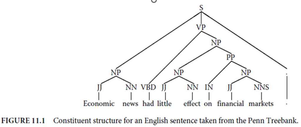
1.       Explain constituent structure and dependency structure for an English sentence with a neat diagram with respect to Syntactic Representations of Statistical Parsing.

2.       Write in brief about Statistical Parsing Models. Also, explain Parser Evaluation in Statistical Parsing.

3.       How PCFGs work as Statistical Parsing Models? Explain with a neat diagram.

4.       Describe Generative Models. Also compare it with PCFG model.

5.       Describe History-Based Models in detail.

6.       Write a brief note on PCFG Transformations.

7.       Describe the standard version of Data-Oriented Parsing in detail.

8.       Explain the working of Local Discriminative Models in detail.

9.       Explain the working of Global Discriminative Models in detail.

10.   Explain in brief about Beyond Supervised Parsing, Weakly Supervised Parsing and unsupervised parsing.

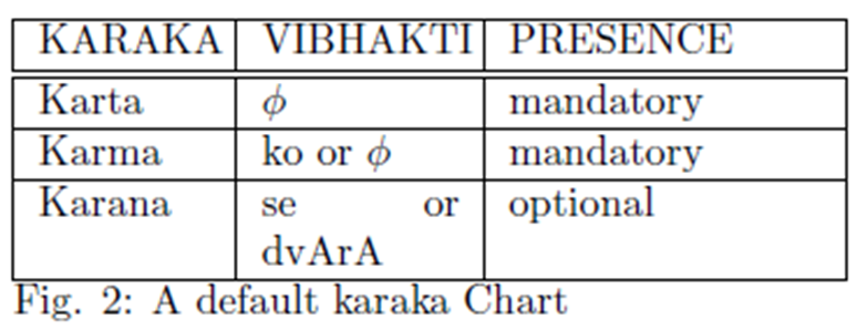
11.   What is Indian Language Parsing in Paninian Karaka Theory? Explain with respect to a default karaka chart and transformation rules.

12.   What is constraint-based parsing? Explain in detail with respect to Paninian Karaka Theory.

13.   What is malt-parsing? Explain in brief with respect to Inductive Dependency Parsing.

14.   Write a brief note on Parsing Algorithms of malt parsing.

15.   Explain Feature Models in brief with respect to malt parsing.

16.   What is Learning Algorithms in malt parsing? Also write about Learning and Parsing.

Unit 5

1.       What is MWEs? Explain Linguistic Properties of MWEs Idiomaticity property of its in detail.

2.       Describe Lexical Idiomaticity and statistic Idiomaticity of MWEs.

3.       Describe Syntactic Idiomaticity and Semantic Idiomaticity of MWEs.

4.       Describe Lexical Idiomaticity and Pragmatic Idiomaticity of MWEs.

5.       How to Test an Expression for MWEhood? Explain in detail.

6.       What are the Types of MWEs? Explain Verbal MWEs in detail.

7.       What are the Types of MWEs? Explain Nominal MWEs and Prepositional MWEs in detail.

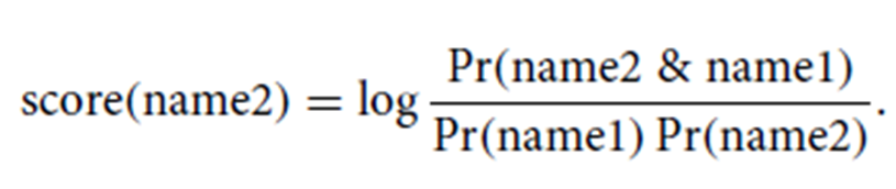
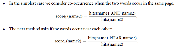
8.       Why do we use normalized web distance? Explain any two methods of it.

9.       Explain Association Measures and Attributes methods for Word Similarity.

10.   Describe Relational Word Similarity and Latent Semantic Analysis methods for Word Similarity.

11.   What is Kolmogorov Complexity? Explain in brief.

12.   Define Information Distance. Also explain Normalized Information Distance.

13.   Define Information Distance. Also explain Normalized Compression Distance.

14.   Write a brief note on Applications and Experiments of Normalized word

NLP Lab Manual

https://medium.com/nerd-for-tech/text-summarization-with-machine-and-deep-learning-in-python-4fbaf5cf746b

Practical No. 1:

a)      Install NLTK


Python 3.9.2 Installation on Windows


Step 1) Go to link https://www.python.org/downloads/and select the latest version for windows.


Note: If you don't want to download the latest version, you can visit the download tab and see all releases.


Step 2) Click on the Windows installer (64 bit)


Step 3) Select Customize Installation


Step 4) Click NEXT


Step 5) In next screen

1.      Select the advanced options

2.      Give a Custom install location. Keep the default folder as c:\Program files\Python39

3.      Click Install


Step 6) Click Close button once install is done.


Step 7) open command prompt window and run the following commands:

C:\Users\Beena Kapadia>pip install --upgrade pip

C:\Users\Beena Kapadia> pip install --user -U nltk

C:\Users\Beena Kapadia> >pip install --user -U numpy

C:\Users\Beena Kapadia>python

>>> import nltk

>>> 


(Browse https://www.nltk.org/install.html for more details)


b) Convert the given text to speech.

Source code:


# text to speech


# pip install gtts

# pip install playsound


from playsound import playsound


# import required for text to speech conversion


from gtts import gTTS

mytext = "Welcome to Natural Language programming"

language = "en"

myobj = gTTS(text=mytext, lang=language, slow=False)

myobj.save("myfile.mp3")

playsound("myfile.mp3")


Output:

welcomeNLP.mp3 audio file is getting created and it plays the file with playsound() method, while running the program.


c) Convert audio file Speech to Text.

Source code:


Note: required to store the input file "male.wav" in the current folder before running the program.


#pip3 install SpeechRecognition pydub


import speech_recognition as sr

filename = " the most frequent noun "


# initialize the recognizer

r = sr.Recognizer()


# open the file

with sr.AudioFile(filename) as source:

    # listen for the data (load audio to memory)

    audio_data = r.record(source)

    # recognize (convert from speech to text)

    text = r.recognize_google(audio_data)

    print(text)


Input:

male.wav (any wav file)


Output:


Practical No. 2:

a. Study of various Corpus – Brown, Inaugural, Reuters, udhr with various methods like filelds, raw, words, sents, categories.

b. Create and use your own corpora (plaintext, categorical)

c. Study of tagged corpora with methods like tagged_sents, tagged_words.

d. Write a program to find the most frequent noun tags.


2 a. Study of various Corpus – Brown, Inaugural, Reuters, udhr with various methods like fields, raw, words, sents, categories,

source code:

'''NLTK includes a small selection of texts from the Project brown electronic text archive, which contains some 25,000 free electronic books, hosted at http://www.brown.org/. We begin by getting the Python interpreter to load the NLTK package, then ask to see nltk.corpus.brown.fileids(), the file identifiers in this corpus:'''


import nltk


from nltk.corpus import brown

print ('File ids of brown corpus\n',brown.fileids())


'''Let’s pick out the first of these texts — Emma by Jane Austen — and give it a short name, emma, then find out how many words it contains:'''

ca01 = brown.words('ca01')


# display first few words

print('\nca01 has following words:\n',ca01)


# total number of words in ca01

print('\nca01 has',len(ca01),'words')


#categories or files

print ('\n\nCategories or file in brown corpus:\n')

print (brown.categories())


'''display other information about each text, by looping over all the values of fileid corresponding to the brown file identifiers listed earlier and then computing statistics for each text.'''

print ('\n\nStatistics for each text:\n')

print ('AvgWordLen\tAvgSentenceLen\tno.ofTimesEachWordAppearsOnAvg\t\tFileName')

for fileid in brown.fileids():

    num_chars = len(brown.raw(fileid))

    num_words = len(brown.words(fileid))

    num_sents = len(brown.sents(fileid))

    num_vocab = len(set([w.lower() for w in brown.words(fileid)]))

    print (int(num_chars/num_words),'\t\t\t', int(num_words/num_sents),'\t\t\t', int(num_words/num_vocab),'\t\t\t', fileid)


output:

b.  Create and use your own corpora (plaintext, categorical)

source code:

'''NLTK includes a small selection of texts from the Project filelist electronic text archive, which contains some 25,000 free electronic books, hosted at http://www.filelist.org/. We begin by getting the Python interpreter to load the NLTK package, then ask to see nltk.corpus.filelist.fileids(), the file identifiers in this corpus:'''


import nltk

from nltk.corpus import PlaintextCorpusReader


corpus_root = 'D:/2020/NLP/Practical/uni'

filelist = PlaintextCorpusReader(corpus_root, '.*')

print ('\n File list: \n')

print (filelist.fileids())


print (filelist.root)


'''display other information about each text, by looping over all the values of fileid corresponding to the filelist file identifiers listed earlier and then computing statistics for each text.'''

print ('\n\nStatistics for each text:\n')

print ('AvgWordLen\tAvgSentenceLen\tno.ofTimesEachWordAppearsOnAvg\tFileName')

for fileid in filelist.fileids():

    num_chars = len(filelist.raw(fileid))

    num_words = len(filelist.words(fileid))

    num_sents = len(filelist.sents(fileid))

    num_vocab = len(set([w.lower() for w in filelist.words(fileid)]))

    print (int(num_chars/num_words),'\t\t\t', int(num_words/num_sents),'\t\t\t', int(num_words/num_vocab),'\t\t', fileid)


output:


c. Study of tagged corpora with methods like tagged_sents, tagged_words.


Source code:

import nltk

from nltk import tokenize

nltk.download('punkt')

nltk.download('words')


para = "Hello! My name is Beena Kapadia. Today you'll be learning NLTK."

sents = tokenize.sent_tokenize(para)

print("\nsentence tokenization\n===================\n",sents)


# word tokenization

print("\nword tokenization\n===================\n")

for index in range(len(sents)):

  words = tokenize.word_tokenize(sents[index])

  print(words)


output:


d. Write a program to find the most frequent noun tags.

Code:

import nltk

from collections import defaultdict

nltk.download('punkt')

nltk.download('averaged_perceptron_tagger')

text = nltk.word_tokenize("Nick likes to play football. Nick does not like to play cricket.")

tagged = nltk.pos_tag(text)

print(tagged)


# checking if it is a noun or not

addNounWords = []

count=0

for words in tagged:

    val = tagged[count][1]

    if(val == 'NN' or val == 'NNS' or val == 'NNPS' or val == 'NNP'):

        addNounWords.append(tagged[count][0])

    count+=1


print (addNounWords)


temp = defaultdict(int)


# memoizing count

for sub in addNounWords:

    for wrd in sub.split():

        temp[wrd] += 1


# getting max frequency

res = max(temp, key=temp.get)


# printing result

print("Word with maximum frequency : " + str(res))


output:


3. a. Study of Wordnet Dictionary with methods as synsets, definitions, examples, antonyms

 ‘‘‘ WordNet is the lexical database i.e. dictionary for the English language, specifically designed for natural language processing.

Synset is a special kind of a simple interface that is present in NLTK to look up words in WordNet. Synset instances are the groupings of synonymous words that express the same concept. Some of the words have only one Synset and some have several.’’’

    Source code:

'''WordNet provides synsets which is the collection of synonym words also called “lemmas”'''

import nltk

from nltk.corpus import wordnet

   nltk.download('wordnet')

print(wordnet.synsets("computer"))


# definition and example of the word ‘computer’

print(wordnet.synset("computer.n.01").definition())


#examples

print("Examples:", wordnet.synset("computer.n.01").examples())


#get Antonyms

print(wordnet.lemma('buy.v.01.buy').antonyms())


output:


b. Study lemmas, hyponyms, hypernyms.

Hyponyms and hypernyms are both terms that come under the lexis/semantics section of English language. A hypernym describes a more broad term, for example color. A hyponym is a more specialised and specific word, for example: Purple, Red, Blue, Green would be a hyponym of color.  

    Source code:

import nltk

from nltk.corpus import wordnet

   nltk.download('wordnet')

print(wordnet.synsets("computer"))

print(wordnet.synset("computer.n.01").lemma_names())

#all lemmas for each synset.

for e in wordnet.synsets("computer"):

    print(f'{e} --> {e.lemma_names()}')


#print all lemmas for a given synset

print(wordnet.synset('computer.n.01').lemmas())


#get the synset corresponding to lemma

print(wordnet.lemma('computer.n.01.computing_device').synset())


#Get the name of the lemma

print(wordnet.lemma('computer.n.01.computing_device').name())


#Hyponyms give abstract concepts of the word that are much more specific

#the list of hyponyms words of the computer


syn = wordnet.synset('computer.n.01')

print(syn.hyponyms)


print([lemma.name() for synset in syn.hyponyms() for lemma in synset.lemmas()])


#the semantic similarity in WordNet

vehicle = wordnet.synset('vehicle.n.01')

car = wordnet.synset('car.n.01')


print(car.lowest_common_hypernyms(vehicle))


    Output:


c) sentence tokenization, word tokenization, Part of speech Tagging and chunking of user defined text.

Source code:

import nltk

from nltk import tokenize

nltk.download('punkt')

from nltk import tag

from nltk import chunk

nltk.download('averaged_perceptron_tagger')

nltk.download('maxent_ne_chunker')

nltk.download('words')


para = "Hello! My name is Beena Kapadia. Today you'll be learning NLTK."

sents = tokenize.sent_tokenize(para)

print("\nsentence tokenization\n===================\n",sents)


# word tokenization

print("\nword tokenization\n===================\n")

for index in range(len(sents)):

  words = tokenize.word_tokenize(sents[index])

  print(words)


# POS Tagging

tagged_words = []

for index in range(len(sents)):

  tagged_words.append(tag.pos_tag(words))

print("\nPOS Tagging\n===========\n",tagged_words)


# chunking

tree = []

for index in range(len(sents)):

  tree.append(chunk.ne_chunk(tagged_words[index]))

print("\nchunking\n========\n")

print(tree)


Output:

sentence tokenization

===================

 ['Hello!', 'My name is Beena Kapadia.', "Today you'll be learning NLTK."]


word tokenization

===================


['Hello', '!']

['My', 'name', 'is', 'Beena', 'Kapadia', '.']

['Today', 'you', "'ll", 'be', 'learning', 'NLTK', '.']


POS Tagging

===========

 [[('Today', 'NN'), ('you', 'PRP'), ("'ll", 'MD'), ('be', 'VB'), ('learning', 'VBG'), ('NLTK', 'NNP'), ('.', '.')], [('Today', 'NN'), ('you', 'PRP'), ("'ll", 'MD'), ('be', 'VB'), ('learning', 'VBG'), ('NLTK', 'NNP'), ('.', '.')], [('Today', 'NN'), ('you', 'PRP'), ("'ll", 'MD'), ('be', 'VB'), ('learning', 'VBG'), ('NLTK', 'NNP'), ('.', '.')]]


chunking

========


[Tree('S', [('Today', 'NN'), ('you', 'PRP'), ("'ll", 'MD'), ('be', 'VB'), ('learning', 'VBG'), Tree('ORGANIZATION', [('NLTK', 'NNP')]), ('.', '.')]), Tree('S', [('Today', 'NN'), ('you', 'PRP'), ("'ll", 'MD'), ('be', 'VB'), ('learning', 'VBG'), Tree('ORGANIZATION', [('NLTK', 'NNP')]), ('.', '.')]), Tree('S', [('Today', 'NN'), ('you', 'PRP'), ("'ll", 'MD'), ('be', 'VB'), ('learning', 'VBG'), Tree('ORGANIZATION', [('NLTK', 'NNP')]), ('.', '.')])]


       4. a) Named Entity recognition using user defined text.

Source code:

!pip install -U spacy

!python -m spacy download en_core_web_sm

import spacy


# Load English tokenizer, tagger, parser and NER

nlp = spacy.load("en_core_web_sm")


# Process whole documents

text = ("When Sebastian Thrun started working on self-driving cars at "

        "Google in 2007, few people outside of the company took him "

        "seriously. “I can tell you very senior CEOs of major American "

        "car companies would shake my hand and turn away because I wasn’t "

        "worth talking to,” said Thrun, in an interview with Recode earlier "

        "this week.")

doc = nlp(text)


# Analyse syntax

print("Noun phrases:", [chunk.text for chunk in doc.noun_chunks])

print("Verbs:", [token.lemma_ for token in doc if token.pos_ == "VERB"])


Output:

Noun phrases: ['Sebastian Thrun', 'self-driving cars', 'Google', 'few people', 'the company', 'him', 'I', 'you', 'very senior CEOs', 'major American car companies', 'my hand', 'I', 'Thrun', 'an interview', 'Recode']

Verbs: ['start', 'work', 'drive', 'take', 'tell', 'shake', 'turn', 'be', 'talk', 'say']


b) Named Entity recognition with diagram using NLTK corpus – treebank.

Source code:


Note: It runs on Python IDLE


import nltk

nltk.download('treebank')

from nltk.corpus import treebank_chunk

treebank_chunk.tagged_sents()[0]


treebank_chunk.chunked_sents()[0]

treebank_chunk.chunked_sents()[0].draw()


Output:


       5.  a) Implementation of Deductive Chart Parsing using context free grammar and a given sentence – Book that flight


Source code:

import nltk

from nltk import tokenize

grammar1 = nltk.CFG.fromstring("""

            S -> VP

        VP -> VP NP

        NP -> Det  NP

        Det -> 'that'

        NP -> singular Noun

        NP -> 'flight'

        VP -> 'Book' 

            """)

sentence = "Book that flight"


nltk.download('punkt')


for index in range(len(sentence)):

    all_tokens = tokenize.word_tokenize(sentence)

print(all_tokens)


parser = nltk.ChartParser(grammar1)

for tree in parser.parse(all_tokens):

    print(tree)

    tree.draw()


output:


b) Implementation of Deductive Chart Parsing using context free grammar and a given sentence - "I saw a bird in my balcony"


Source code:

import nltk

from nltk import tokenize

grammar1 = nltk.CFG.fromstring("""

S -> NP VP

PP -> P NP

NP -> Det N | Det N PP | 'I'

VP -> V NP | VP PP

Det -> 'a' | 'my'

N -> 'bird' | 'balcony'

V -> 'saw'

P -> 'in'

""")

sentence = "I saw a bird in my balcony"


for index in range(len(sentence)):

  all_tokens = tokenize.word_tokenize(sentence)

print(all_tokens)


# all_tokens = ['I', 'saw', 'a', 'bird', 'in', 'my', 'balcony']

parser = nltk.ChartParser(grammar1)

for tree in parser.parse(all_tokens):

    print(tree)

    tree.draw()


output:


6.         a) Analyzing the meaning of sentence by querying a database. Find the cities of India by applying a query - 'What cities are located in India' and the context free grammar from the file 'sqlIndia.fcfg'. Hint: sqlIndia.fcfg file should be in the same folder.


Source code:

#Analysing the meaning of sentence by querying a database

# show CFG

# pip install nltk

import nltk

nltk.data.show_cfg('sqlIndia.fcfg')


# Convert into bracket (list] form

from nltk.parse import load_parser

cp = load_parser('sqlIndia.fcfg')

query = 'What cities are located in India'

trees = list(cp.parse(query.split()))

print (trees)


# generate query as a sentence with punctuations (,)

answer = trees[0].label()['SEM']

print (answer)


# generate query as tokens

answer = [s for s in answer if s]


#join all tokens

q = ' '.join(answer)

print (q)


## TILL NOW WE HAVE CONVERTED NLP STAEMENT INTO DATABASE STATEMENT ##


# Finally, we execute the query over the database city.db and retrieve some results:

from nltk.sem import chat80

nltk.download('city_database')


# apply query q to city.db

rows = chat80.sql_query('corpora/city_database/city.db', q)


# print cities

for r in rows:

    print (r)       


output:


b. # Building a Discourse Representation Theory(DRT) by parsing a string representation - Angus owns a dog.


Source code:

# e.g.'Angus owns a dog'.

# A discourse representation structure (DRS) presents the meaning of discourse.


# parse a string and represent Discourse Representation Structure

import nltk

read_the_expr = nltk.sem.DrtExpression.fromstring


drs1 = read_the_expr('([x, y], [Angus(x), dog(y), own(x, y)])')

print(drs1)

drs1.draw()


# every DRS can be translated into a formula of first-order logic, and the fol() method implements this translation.

print(drs1.fol())


# In order to parse with grammar drt.fcfg, we specify in the call to load_parser() that SEM values in feature structures are to be parsed using DrtParser.

from nltk import load_parser

parser = load_parser('grammars/book_grammars/drt.fcfg', logic_parser=nltk.sem.drt.DrtParser())

trees = list(parser.parse('Angus owns a dog'.split()))

print(trees[0].label()['SEM'].simplify())

trees[0].draw()


output:


7.         Study PorterStemmer, LancasterStemmer, RegexpStemmer, SnowballStemmer

and WordNetLemmatizer


Code:

# PorterStemmer

import nltk

from nltk.stem import PorterStemmer

word_stemmer = PorterStemmer()

print(word_stemmer.stem('writing'))

Output:

                #LancasterStemmer

import nltk

from nltk.stem import LancasterStemmer

Lanc_stemmer = LancasterStemmer()

print(Lanc_stemmer.stem('writing'))

Output:

#RegexpStemmer

import nltk

from nltk.stem import RegexpStemmer

Reg_stemmer = RegexpStemmer('ing$|s$|e$|able$', min=4)

print(Reg_stemmer.stem('writing'))


output


#SnowballStemmer

import nltk

from nltk.stem import SnowballStemmer

english_stemmer = SnowballStemmer('english')

print(english_stemmer.stem ('writing'))


output


#WordNetLemmatizer

from nltk.stem import WordNetLemmatizer


lemmatizer = WordNetLemmatizer()


print("word :\tlemma") 

print("rocks :", lemmatizer.lemmatize("rocks"))

print("corpora :", lemmatizer.lemmatize("corpora"))


# a denotes adjective in "pos"

print("better :", lemmatizer.lemmatize("better", pos ="a"))


Output:


8          a) Parse a sentence - "old men and women" and draw a tree using probabilistic parser

Source code:

import nltk

from nltk import PCFG


grammar = PCFG.fromstring('''

NP -> NNS [0.5] | JJ NNS [0.3] | NP CC NP [0.2]

NNS -> "men" [0.1] | "women" [0.2] | "children" [0.3] | NNS CC NNS [0.4]

JJ -> "old" [0.4] | "young" [0.6]

CC -> "and" [0.9] | "or" [0.1]

''')


print(grammar)

viterbi_parser = nltk.ViterbiParser(grammar)

token = "old men and women".split()

obj = viterbi_parser.parse(token)


print("Output: ")

for x in obj:

    print(x)


Output:


b). Malt parsing:

               Parse a sentence - 'I saw a bird from my window.' and draw a tree using malt parsing.

Note:   1) Java should be installed.

2) maltparser-1.7.2 zip file should be copied in C:\Users\Beena  Kapadia\AppData\Local\Programs\Python\Python39 folder and should be extracted in the same folder.

3) engmalt.linear-1.7.mco file should be copied to C:\Users\Beena  Kapadia\AppData\Local\Programs\Python\Python39 folder

Source code:

# copy maltparser-1.7.2(unzipped version) and engmalt.linear-1.7.mco files to C:\Users\Beena Kapadia\AppData\Local\Programs\Python\Python39 folder

# java should be installed

# environment variables should be set - MALT_PARSER - C:\Users\Beena Kapadia\AppData\Local\Programs\Python\Python39\maltparser-1.7.2 and MALT_MODEL - C:\Users\Beena Kapadia\AppData\Local\Programs\Python\Python39\engmalt.linear-1.7.mco


from nltk.parse import malt

mp = malt.MaltParser('maltparser-1.7.2', 'engmalt.linear-1.7.mco')#file       

t = mp.parse_one('I saw a bird from my window.'.split()).tree()

print(t)

t.draw()


Output:

(saw I (bird a (from (window. my))))


9.   a) Multiword Expressions in NLP for multiword – ‘New Delhi’ in '''Good cake cost Rs.1500\kg in New Delhi.  Please buy me one of them.\n\nThanks.'''


Source code:

# Multiword Expressions in NLP


from nltk.tokenize import MWETokenizer

from nltk import sent_tokenize, word_tokenize

s = '''Good cake cost Rs.1500\kg in New Delhi.  Please buy me one of them.\n\nThanks.'''

mwe = MWETokenizer([('New', 'Delhi'), ('New', 'York'), ('Hong', 'Kong')], separator='_')

for sent in sent_tokenize(s):

    print(mwe.tokenize(word_tokenize(sent)))


Output:


b) Word Sense Disambiguation for the keyword ‘jam’ in the sentences - 'This device is used to jam the signal' and 'I am stuck in a traffic jam'. Also, for the keyword ‘book’ in the sentences - 'I love reading books on coding.' and 'The table was already booked by someone else.'


Source code:

#Pr 9 b WSD

#The purpose of WSD is to accurately understand the meaning of a word in particular usage or sentence, it can be used for the correct labeling of words.

from nltk.wsd import lesk

from nltk.tokenize import word_tokenize


import nltk

nltk.download('punkt')

nltk.download('wordnet')


a1= lesk(word_tokenize('This device is used to jam the signal'),'jam')

print(a1,a1.definition())

a2 = lesk(word_tokenize('I am stuck in a traffic jam'),'jam')

print(a2,a2.definition())


b1=lesk(word_tokenize('I love reading books on coding.'),'book')

print(b1,b1.definition())

b2 = lesk(word_tokenize('The table was already booked by someone else.'),'book')

print(b2,b2.definition())


Output:


Comments